
The Data: What 13C Tells Us
The Global View
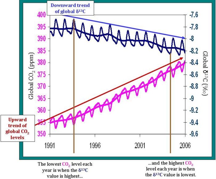
The relative proportion of 13C in our atmosphere is steadily decreasing over time. Before the industrial revolution, δ13C of our atmosphere was approximately -6.5‰; now the value is around -8‰. Recall that plants have less 13C relative to the atmosphere (and therefore have a more negative δ13C value of around -25‰). Most fossil fuels, like oil and coal, which are ancient plant and animal material, have the same δ13C isotopic fingerprint as other plants. The annual trend–the overall decrease in atmospheric δ13C–is explained by the addition of carbon dioxide to the atmosphere that must come from the terrestrial biosphere and/or fossil fuels. In fact, we know from Δ14C measurements, inventories, and other sources, that this decrease is from fossil fuel emissions, and is an example of the Suess Effect.
- Recall that the Suess Effect is the observed decrease in δ13C and Δ14C values due to fossil fuel emissions, which are depleted in 13C and do not contain 14C.
Total atmospheric carbon dioxide levels (not isotopic ratios, but just total carbon dioxide) show strong seasonal variations. In the summer (in the northern hemisphere–where most of the Earth's land sits), carbon dioxide decreases as it is fixed by plants via photosynthesis. In the fall and winter, carbon dioxide increases as many plants stop photosynthesizing and some of the carbon dioxide they fixed is released through respiration from plants, animals, and soils. Seasonal δ13C variations show the opposite pattern. δ13C increases in the summer and decreases in the winter, as you can see on the graph below. This opposite trend is termed anticorrelation, and is explained using the same reasoning behind the total carbon dioxide pattern. When plants take up carbon dioxide, they prefer 12C over 13C. This leaves relatively more 13C in the atmosphere, which increases the δ13C of the atmosphere. However, in the winter, when the plants release more carbon dioxide than they consume, this carbon dioxide entering the atmosphere is relatively poor in 13C. This decreases the δ13C of the atmosphere during the fall and winter of each year since the carbon dioxide released from the plants is relatively rich in 12C–decreasing the ratio of 13C to 12C in the atmosphere. Of course, the seasons are opposite in the Northern and Southern Hemispheres, so why don't the trends in the two hemispheres cancel each other out? The answer is as easy as looking at a globe. There's a lot more land and a lot more land biota in the Northern Hemisphere, so on average across the globe, the δ13C and CO2 change with the Northern Hemisphere seasons.
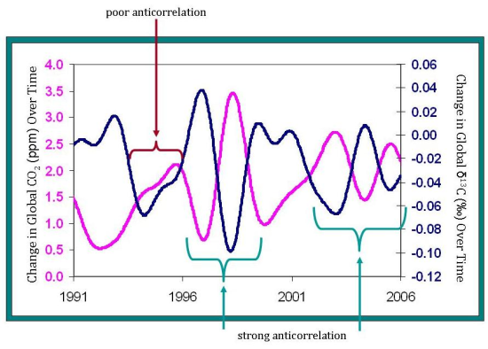
One of the most important uses of δ13C measurements is in determining the strength of the terrestrial biosphere sink. Since about half of the carbon dioxide we add to the atmosphere each year is absorbed into various sinks, it is important for future predictions to know where exactly that carbon dioxide goes. Scientists look at the rate of change of carbon dioxide levels–how fast carbon dioxide levels are increasing or decreasing. This can be compared to the rate of change of δ13C levels. The strong anticorrelation seen between these two rates tells NOAA scientists that, globally, the terrestrial biosphere responds to atmospheric carbon dioxide levels. For example, when carbon dioxide is added to the atmosphere at an increased rate, often the terrestrial biosphere will take up carbon dioxide at an increased rate as well. However, although the terrestrial biosphere is currently responding to changes in the rate of carbon dioxide released from sources, it is unclear if this will continue into the future. How long will the terrestrial biosphere be able to respond before it reaches its capacity–or will it?
Notice also, that the δ13C is not always perfectly anticorrelated with changes in atmospheric carbon dioxide. A time when this anticorrelation is less prevalent is from 1995-1996. During this period, another process must be involved in controlling carbon dioxide levels. Perhaps oceanic uptake fluctuated more during this period, but was relatively constant during the rest of time shown on the graph.
Comparing Local Views
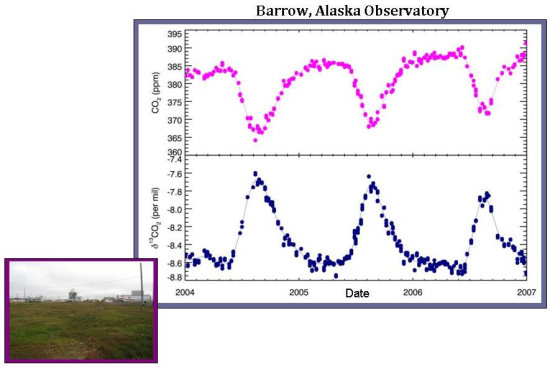
At a local scale, δ13C measurements show how much of the seasonal fluctuations are controlled by the terrestrial biosphere versus oceanic exchange. The differences among sites are best exemplified by comparing a sample site located in Barrow, Alaska with the South Pole air sampling site. In Barrow, there are very large differences in carbon dioxide on a seasonal basis, which is (nearly perfectly) anticorrelated with the δ13C of carbon dioxide. As discussed in the global trend, this means that the atmospheric carbon dioxide seasonality in Barrow is controlled almost entirely by the terrestrial biosphere. Oceanic exchange–which would affect total carbon dioxide but not δ13C–appears to play little to no role in determining overall CO2 levels at Barrow.
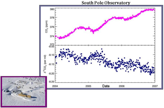
In comparison, there is only a weak anticorrelation between atmospheric carbon dioxide and δ13C values at the South Pole. This implies that terrestrial uptake plays only a small role in atmospheric CO2 levels, and, instead, another process is involved. Perhaps this other process is oceanic uptake. In any case, it makes reasonable sense that at the South Pole, which is devoid of plants, the role of the terrestrial biosphere is greatly diminished.
“Disequilibrium Fluxes”
While the two main categories of fluxes that δ13C helps to distinguish are fluxes from either (1) the terrestrial biosphere or (2) fluxes from the ocean, to determine the relative strength of carbon sources and sinks, these two fluxes must be further separated. Mainly, it is important to remember that the current fluxes from these two sinks are related to the atmospheric composition at the time that the carbon was stored. However, the δ13C of fluxes into these pools are determined by the current atmospheric composition. Although the amount of time carbon is stored (the turnover time) varies greatly, it is much less in the terrestrial biosphere than in the ocean. On land, carbon is often stored between several years or several hundred years. Say, though, that a tree that is thirty years old dies. The carbon released from the tree will have a different δ13C fingerprint than trees growing today. Because the atmosphere has become more depleted in 13C over time, the δ13C of the carbon released from the dead tree will be higher than the δ13C of living trees taking in carbon dioxide from today's atmosphere.
A similar logic holds for oceanic fluxes, but to a greater extent. While the turnover time in the terrestrial biosphere is tens-to-hundreds of years, the turnover time in the ocean ranges from hundreds-to-thousands of years. Since there was not yet any carbon from fossil fuel in the atmosphere 1,000 years ago, the atmospheric δ13C was even higher (about -7‰). Therefore, the flux from the ocean has a less negative δ13C than the current flux into the ocean. The difference in these two fluxes (between -10‰ going into the ocean and -9.5‰ for the carbon coming out of the ocean) is greater than the differences in the terrestrial fluxes (only about 0.3‰) because of the longer turnover time in the ocean. Knowing the differences between the fluxes into and out of each pool helps scientists at NOAA better understand the carbon cycle and the strength of each source and sink of atmospheric carbon dioxide.

 Previous
