Stage 2 - Applying Sprior sigma to H Slices and Calculating HQ¶

The modification that NOAA made to the method of Yadav and Michalak uses time and space varying values for $\sigma^2$ in equation 2.

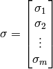
Define a vector $\sigma$ :

$\sigma = \begin{bmatrix} \sigma_1 \\ \sigma_2 \\ \vdots \\ \sigma_m \end{bmatrix}$

and a matrix $I_\sigma$ :

$I_\sigma = \begin{bmatrix} \sigma_1 & \dots & 0 \\ \vdots & \dotsi & \vdots \\ 0 & \dots & \sigma_m \end{bmatrix}$

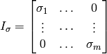
where m=p✕r = (number of time steps) ✕ (number of spatial grid cells).

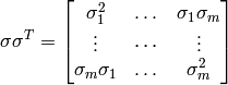
Then

$\sigma \sigma^T = \begin{bmatrix} \sigma_1^2 & \dots & \sigma_1\sigma_m \\ \vdots & \dotsi & \vdots \\ \sigma_m\sigma_1 & \dots & \sigma_m^2 \end{bmatrix}$

The prior error covariance is modeled with temporal decorrelation described by the p✕p matrix D and spatial decorrelation described by the r✕r matrix E such that:

$Q = \left(\sigma \sigma^T\right) \times \left(D \otimes E\right) = I_\sigma\left(D \otimes E \right)I_\sigma$

where $\times$ denotes element by element multiplication and $\otimes$ denotes the Kronecker product.

The modified algorithm for computing HQ is described by:

(1) $HQ = \left[\left( \left( \sum_{i=1}^{p} d_{i1}h_iI_{\sigma_i}\right)EI_{\sigma_1}\right) \left( \left( \sum_{i=1}^{p} d_{i2}h_iI_{\sigma_i}\right)EI_{\sigma_2}\right) ... \left( \left( \sum_{i=1}^{p} d_{iq}h_iI_{\sigma_i}\right)EI_{\sigma_q}\right)\right]$

where the diagonal of $I\sigma_i$ is the portion of the the vector $\sigma$ corresponding to a single timestep $i$ . Compare to Equation (9) from Yadav and Michalak (2012). The algorithm speed can be greatly improved if $h_iI_{\sigma_i}$ for each time step is pre-computed and retrieved as needed. We call this pre-computed $h_iI_{\sigma_i}$ Hsigma.

Hsigma¶

Hsigma requires multiplying the H strip for each timestep by the corresponding sigma values for that time step. The modified H strip is then saved for later use in the HQ calculations.

Sigma File Format¶

The format of the sigma file can be either a numpy .npy file with dimensions ntimesteps x nlandcells, or a netcdf file with a variable named ‘sigma’, with the dimensions ntimesteps x nlats x nlons. The lat and lon dimensions must match what is defined in the configuration file.

Example:

ncdump -h sigma.nc

netcdf sigma {
dimensions:
        dates = 92 ;
        lat = 70 ;
        lon = 120 ;
variables:
        float dates(dates) ;
                string dates:long_name = "days since 2000-01-01" ;
                string dates:units = "days since 2000-01-01" ;
        double lat(lat) ;
                string lat:units = "degrees_north" ;
                string lat:long_name = "latitude" ;
                string lat:description = "latitude of center of cells" ;
        double lon(lon) ;
                string lon:units = "degrees_east" ;
                string lon:long_name = "longitude" ;
                string lon:description = "longitude of center of cells" ;
        float sigma(dates, lat, lon) ;
                string sigma:lonFlip = "longitude coordinate variable has been reordered via lonFlip" ;
                string sigma:long_name = "N2O emissions" ;
                string sigma:units = "nmolN2O/m2/s" ;
                sigma:time = 335.f ;
                string sigma:comment = "from CTlagrange/create_sprior_n2oES.ncl" ;
                sigma:_FillValue = 9.96921e+36f ;
}

Usage¶

hsigma.py is run with:

python hsigma.py [-c configfile] [-b] sigmafile

where
        sigmafile  : file with sprior uncertainty values.  Can be either a numpy save file of dimension ntimesteps x ncells,
                     or a netcdf file with 'sigma' variable of dimensions ntimesteps x nlat x nlon
        configfile : configuration file. If not specified, use 'config.ini'.
        -b : write H files in binary format. Default is a numpy savez file.

Required input files:
        H slice files

Output¶

hsigma.py creates another set of H slice files in the directory ‘Hsigma’, corresponding to the original H slice files. The -b option will produce binary formatted files, otherwise they are in numpy savez .npz format.

HQ Calculations¶

The script hq.py is used to calculate the HQ part of equation 1. It requires for input the spatial distance array (see section Spatial Distances) and the hsigma slice files created with hsigma.py. Equation 2 uses a parameter l_t for specifying the temporal covariance D. In the inversion code, a constant value of l_t is used, and is defined in the configuration file with key name ‘temporal_corr_length’. The units for this value are in days.

Example:

temporal_corr_length = 7.0

The output from hq.py are HQ slice files, and $HQH^T$ matrix from equation 1.

Usage¶

hq.py is run with:

hq.py [-m] [-c configfile] receptor_file sigmafile

where
        receptor_file : file containing footprint file names, 1 line per receptor
        sigmafile     : file with sprior uncertainty values.  Can be either a numpy save file of dimension ntimesteps x ncells,
                        or a netcdf file with 'sigma' variable of dimensions ntimesteps x nlat x nlon
        -m            : split computation into confg['nprocs'] threads, otherwise use single process.
        -c configfile : configuration file. If not specified, use 'config.ini'.

Required input files:
        hsigma slice files
        spcov.npy - spatial distance file

Output
        HQ slice files
        HQHT array