Stage 4 - Inversion and posterior uncertainty¶

Inversion¶

Once the HQ Calculations and Stage 3 - Observations, background and priors steps are completed, the final inversion step can be done. The user needs to also supply the values of the diagonal of R.

The program inversion.py performs the calculations, and makes several output files,

shat.npy, shat.nc - The calculated $\hat{s}$ , both in numpy save format and netcdf format.

hshat.txt - $\hat{s}$ convolved with H

hqhti.npy - Result of $(HQH^T + R)^{-1}$ from Equation 1.

hqht_zhsp.npy - Result of $(HQH^T + R)^{-1} * (z-Hs_p)$ from Equation 1.

qhts.npy - The result of $(HQ)^T * (HQH^T + R)^{-1} * (z-Hs_p)$ from Equation 1.

Prerequisites¶

R values - Variances of model data mismatch.

sprior - contains s_p. Can be either a numpy save file, dimensions (ntimesteps x ncells), or a netcdf file, with a variable named ‘sprior’ and dimensions (ntimesteps x nlat x nlon)

HQ blocks created by hq.py.

HQHT array created by hq.py.

zhsp.txt created by make_z.py.

Usage¶

inversion.py is run with:

inversion.py [-c configfile] [-b] spriorfile rfile

where

   Required arguments
        spriorfile : file name with sprior data
        rfile : file name with R data

   Optional arguments
        -c : Specify the configuration file to use. Default is 'config.ini'.
        -b : If set, use boundary value optimization files.

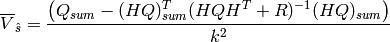
Posterior uncertainty¶

The uncertainty covariance of the estimated $\hat{s}$ can be written as:

(1) $V_{\hat{s}} = Q - (HQ)^T (HQH^T + R)^{-1} HQ$

The a posteriori covariance matrix $V_{\hat{s}}$ is a computational bottlenect for large inverse problems. Instead, the a posteriori covariance is calculated directly at aggregated scales, without explicitly calculating $V_{\hat{s}}$ . The estimated aggregated grid-scale $\overline{V_{\hat{s}}}$ averaged over desired time periods is:

(2) $\overline{V}_{\hat{s}} = \frac{\left(Q_{sum} - (HQ)_{sum}^T(HQH^T + R)^{-1}(HQ)_{sum}\right)} {k^2}$

where $k$ is the number of time steps in the aggregated time period. Using a space and time varying $\sigma$ in equation 3, $Q_{sum}$ is defined as

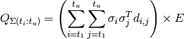
(3) $Q_{\Sigma(t_i:t_u)} = \left(\sum_{i=t_1}^{t_u} \sum_{j=t_1}^{t_u} \sigma_i \sigma_j^T d_{i,j} \right) \times E$

where:

(4) $\sigma_{rx1} = \begin{bmatrix} \sigma_{p=i, r=1} \\ \sigma_{p=i, r=2} \\ \vdots \\ \sigma_{p=i, r=t} \end{bmatrix}$

and $Q_{sum}$ represents the sum of all Q blocks between $t_l$ and $t_u$ . However, greatly increased speed is achieved using the equivalent formulation:

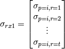
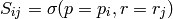
(5) $Q_{\Sigma(t_i:t_u)} = \left(S_{(t_l:t_u)}^T D S_{(t_l:t_u)} \right) \times E$

where $S$ is a p✕r matrix such that:

$S_{ij} = \sigma(p=p_i, r=r_j)$

and $S_{(tl:tu)}$ refers to the portion of S containing timesteps $t_u$ through $t_l$ . As in the constant $\sigma$ case, $(HQ)_{sum}$ is computed simply by summing all of the column blocks of HQ between $t_l$ and $t_u$ .

The time periods for calculating $\overline{V_{\hat{s}}}$ are defined in the configuration file with the key ‘vshat_dates’.

Example:

vshat_dates = ["2012-6-1", "2012-7-1", "2012-8-1", "2012-9-1"]

which will result in estimates for June, July and August of 2012. The time periods are from a date up to but not including the next date. Aggregated posterior uncertainties will also be computed for the entire time span defined in the configuration file with the keys ‘start_date’ and ‘end_date’.

The program apost.py performs the calculations. Output files created are

vshat.npy, vshat.nc - Uncertainty estimates aggregated over the entire time of the inversion, in both npy and netcdf formats.

vshat_month_1.npy, vshat_month_1.nc ... - Uncertainty estimates aggregated over each time period defined in the configuration file.

Usage¶

apost.py is run with:

apost.py [-c configfile] [-b] sigmafile

where

   Required arguments
        sigmafile     : file name with sprior sigma values

   Optional arguments
        -c configfile : Specify the configuration file to use.
        -b            : If set, use boundary value optimization files.