
The Data: What 14C Tells Us
The Global View
Ever since the industrial revolution, the amount of fossil fuels (coal, oil and natural gas) burned around the globe each year has skyrocketed. We humans harness the energy released when we burn fossil fuels for many different needs, but burning fossil fuels also produces carbon dioxide, which is usually released straight into the atmosphere from chimneys, smokestacks, and tailpipes.
- How do we know that this carbon dioxide from fossil fuels has increased the total amount of atmospheric carbon dioxide?
- How do we know how much carbon dioxide is being produced from fossil fuel burning?
Economic Inventories
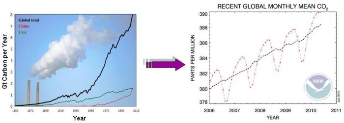
Measurements of CO2 concentration in the atmosphere over time tell us that CO2 is increasing. Countries and industry use economic data to report how much fossil fuel they have burnt each year (such as can be seen above, in the graph on the left), and scientists calculate how much CO2 is produced from the fossil fuels. These tables of data are called inventories. Inventories are, in essence, economic bookkeeping. They are a measurement of the amount of emissions produced from various activities (such as driving a car). From economic inventories and measurements of CO2 in the atmosphere, we know that roughly half of the CO2 from fossil fuel burning stays in the atmosphere. But how accurate are these inventories? It is difficult enough to gather all the required information to make an inventory for a whole country for the year, and even more challenging to make an inventory for a smaller region or a short time period. In a city, for example, we can find out when and how much gasoline was sold at each gas station from sales records. But how can we find out when that gasoline was actually burnt inside the car engine, and emitted the CO2 into the atmosphere?
Isotopic fingerprints and atmospheric measurements are another way to calculate fossil fuel CO2 emissions, and the uncertainties and biases present in self-reporting and inventories are eliminated. While isotopic measurements do contain their own uncertainty, this is quantifiable, and therefore, we can know how much value we should place on the measurements and trends. This differs from self-reporting and inventories. In the near future, the necessity for unbiased reporting may increase if towns, states, and countries are required to reduce emissions 3. Governments or international agencies will be able to track annual emissions for a given region by examining the isotopic content of the surrounding atmosphere; this will help ensure that the area is meeting the emission requirements. These measurements are also important for scientists trying to understand how carbon dioxide exchanges with the terrestrial biosphere and oceans.
14C is the isotope that scientists from NOAA and the University of Colorado use to understand fossil fuel CO2 emissions. You can see how Δ14C values have decreased since 2003 in the background air at Niwot Ridge:
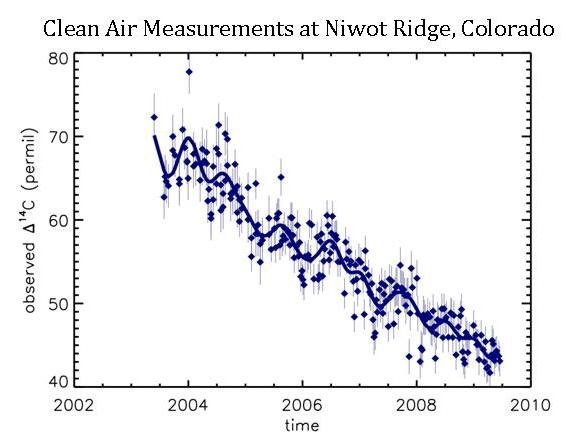
The steady downward trend in Δ14C of background air shows that the additional carbon dioxide added to the atmosphere must have a lower Δ14C value than what is already in the atmosphere. Well, we know that fossil fuels have a Δ14C signal of -1000‰, but that all other sources have a signal that is very close to that of ambient air (approximately + 45‰ in 2010, actually). Therefore, when CO2 from fossil fuels enter the atmosphere, the Δ14C value in the atmosphere goes down. We can precisely calculate how much the Δ14C value in the atmosphere goes down when fossil fuel CO2 is added. It turns out to be about a 3‰ decrease in Δ14C for every 1 ppm of fossil fuel CO2 added to the atmosphere.
But could there be other sources of CO2 that alter Δ14C in the atmosphere? Indeed, there are, but their effects are much smaller than that of fossil fuel CO2. We can see this by comparing maps of modeled global Δ14C levels when looking at all sources or only fossil fuel sources. See how closely the two maps compare? This shows that, by far, the greatest factor altering global Δ14C levels is fossil fuel emissions.
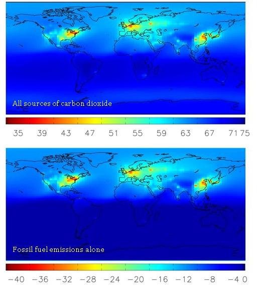
When CO2 is released from the ocean to the atmosphere, it tends to have a Δ14C value slightly lower than the atmosphere, because some of the 14C in it has had time to decay. Over the oceans, and especially in the Southern Hemisphere (which is mostly ocean!) this is the most important effect on Δ14C–as we can see in the lower map of the world. Scientists use measurements of Δ14C in the southern ocean to help understand how fast ocean water “turns over”. Over large land areas though, there are no oceans to release carbon, so the fossil fuel effect is the most important.
However, over the land, there is another effect that we think about – carbon released from plants and soils. Carbon dioxide taken up from the atmosphere by plants is eventually released back to the atmosphere by respiration, but only after a few years (typically 10-20 years). This means that a very small amount of the 14C has decayed away, and the Δ14C value of the CO2 from respiration (when organisms use energy and release carbon dioxide as a byproduct) is different than the atmosphere. Scientists have calculated exactly how much this changes Δ14C in the atmosphere, and it turns out to be not much – to be sure though, when scientists use Δ14C measurements to calculate how much fossil fuel CO2 has been added to the atmosphere, they make a correction for this respiration effect.
A More Local View
Every home heated using natural gas, every coal power plant, and every car powered by gasoline adds some carbon dioxide to the atmosphere. The sum of all the carbon dioxide emitted from these, and many other sources of fossil fuel emissions (and then the mixture of this with background air and CO2 from other sources) is what scientists measure in the “global view.” However, if climate scientists can measure the sum of all the parts, it may come as no surprise that they can measure the parts of the whole. This is exactly what is shown in red on the graph below–the Δ14C measurements caused by carbon dioxide emissions from regional sources of pollution mixed with the background air from samples collected at Tae-Ahn Peninsula in South Korea.
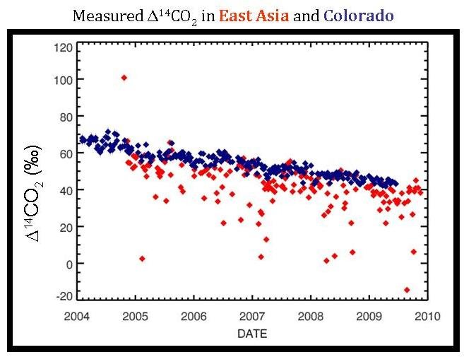
At this point, it may seem odd to have the red data points from TAP on the same graph showing the blue, Niwot Ridge data. The two sites are located half way across the world from each other, so why show both data together? The reason: it is not possible to determine the effect of regional pollution without having a known background level that you can use as a comparison. Since the background level is constantly changing, to accurately determine how the Δ14C level at TAP is affected by pollution, scientists need to compare the data to the background level at that specific date.
Since increased emissions decrease the Δ14C of the air, the extremely low Δ14C red points show where there is a very large regional pollution source. Perhaps a lower Δ14C measurement at TAP occurred during a cold period when a nearby city used a lot of energy to heat the buildings (or, on the flip side, perhaps it was very warm and many people and businesses used their air-conditioning during that time). However, another reason may not actually have anything to do with increased energy consumption, but rather with wind patterns. Some days the wind conditions at TAP bring wind from China; on other days the air comes from Korea. Depending on the difference in energy consumption, the air flasks will show strikingly different Δ14C values depending on the source of the air collected. Therefore, it is very important to know wind conditions on the days that scientists take the air samples. Only then can scientists actually track where the emissions originate and see seasonal and annual changes in regional emissions.
What About that One High Point?
Once you really study the graph comparing Δ14C values for TAP and Niwot Ridge, there is one point that seems very out of place–the TAP measurement that is higher than the background Δ14C levels.
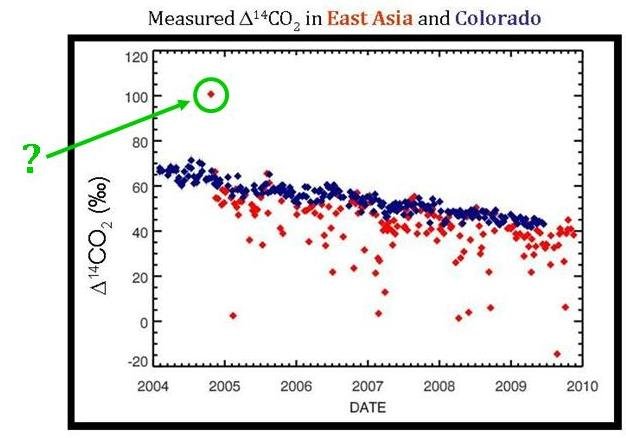
This single point may actually be from a nuclear industry release. Nuclear power has a much higher Δ14C value than the atmosphere (which is what caused the 14C “bomb spike” in the 1960s). Perhaps a nuclear release from North Korea occurred during this time and was recorded in the TAP Δ14C measurements.
To learn more about how Δ14C responds to nuclear energy–and specifically nuclear testing, read The Bomb Spike.
 Previous
