


CarbonTracker Documentation
CT2013 release
CarbonTracker Team
Nov 14, 2014
Contents
1 Introduction1.1 A tool for Science, and Policy
1.2 A Community Effort
1.3 Updates
1.4 Other atmospheric species and their possible roles in constraining the atmospheric carbon budget
2 Oceans Module
2.1 Detailed Description
2.1.1 OIF: the Ocean Inversion Fluxes prior
2.1.2 pCO2-Clim: Takahashi et al. (2009) climatology prior
2.1.3 Gas-transfer velocity and ocean surface properties
2.1.4 Specifics of the Inversion Methodology Related to Air-sea CO2 Fluxes
2.2 Further Reading
3 Terrestrial Biosphere Module
3.1 Detailed Description
3.2 Further Reading
4 Fire Module
4.1 Detailed Description
4.2 Further Reading
5 Observations
5.1 Detailed Description
5.2 Further Reading
6 Fossil Fuel Module
6.1 The "Miller" emissions dataset
6.2 The "ODIAC" emissions dataset
6.3 Uncertainties
6.4 Further Reading
7 Atmospheric Transport
7.1 TM5 offline tracer transport model
7.1.1 ECMWF operational forecast model ("od")
7.1.2 ERA-interim reanalysis model
7.2 Transport metrics
7.2.1 Boundery layer height metrics
7.2.2 Surface SF6 metric
7.2.3 Aircraft SF6 metric
7.2.4 Assimilated CO2 metric
7.2.5 Aircraft CO2 metric
7.3 Further Reading
8 Ensemble Data Assimilation
8.1 Detailed Description
8.1.1 Land-surface classification
8.1.2 Ensemble Size and Localization
8.1.3 Dynamical Model
8.2 Covariance Structure
8.3 Multiple prior models
8.3.1 Posterior Uncertainties in CarbonTracker
8.4 Further Reading
9 Ecoregions in CarbonTracker
9.1 What are ecoregions?
9.2 Why use ecoregions?
9.3 Ecosystems within Transcom regions
9.4 Further Reading
1 Introduction
The goal of the CarbonTracker program is to produce quantitative estimates of atmospheric carbon uptake and release for North America and the rest of the world that are consistent with observed patterns of CO2 in the atmosphere.1.1 A tool for Science, and Policy
CarbonTracker and the associated long-term monitoring of atmospheric CO2 helps improve our understanding of how carbon uptake and release from land ecosystems and oceans are responding to a changing climate, increasing levels of atmospheric CO2 (higher CO2 may enhance plant growth) and other environmental changes, including human management of land and oceans. The open access to all CarbonTracker results means that anyone can scrutinize our work, suggest improvements, and profit from our efforts. This will accelerate the development of a tool that can monitor, diagnose, and possibly predict the behavior of the global carbon cycle, and the climate that is so intricately connected to it. CarbonTracker can become a policy support tool too. Its ability to accurately quantify natural and anthropogenic emissions and uptake at regional scales is currently limited by a sparse observational network. With enough observations, it will become possible to keep track of regional emissions, including those from fossil fuel use, over long periods of time. This will provide an independent check on emissions accounting, estimates of fossil fuel use based on economic inventories. It can thus provide feedback to policies aimed at limiting greenhouse gas emissions. This independent measure of effectiveness of any policy, provided by the atmosphere itself (where CO2 levels matter most), is the bottom line in any mitigation strategy.1.2 A Community Effort
CarbonTracker is intended to be a tool for the community and we welcome feedback and collaboration from anyone interested. Our ability to accurately track carbon with more spatial and temporal detail is dependent on our collective ability to make enough measurements and to obtain enough air samples to characterize variability present in the atmosphere. For example, estimates suggest that observations from tall communication towers (taller than 200m) can tell us about carbon uptake and emission over a radius of only several hundred kilometers. The shows how sparse the current network is. One way to join this effort is by contributing measurements. Regular air samples collected from the surface, towers or aircraft are needed. It would also be very fruitful to expand use of continuous measurements like the ones now being made on very tall (more than 200m) communications towers. Another way to join this effort is by volunteering flux estimates from your own work, to be run through CarbonTracker and assessed against atmospheric CO2. Please contact us if you would like to get involved and collaborate with us.1.3 Updates
CarbonTracker is updated about once per year, generally in the autumn, to include new data and model improvements. The updated calculations are produced for the year 2000 through the most recent complete year of observations. Previous versions are available, and the effect of significant changes to any of the system components is noted.1.4 Other atmospheric species and their possible roles in constraining the atmospheric carbon budget
Many laboratories making high accuracy CO2 observations also make many other measurements of the same air, typically other greenhouse gases such as methane CH4, nitrous oxide N2O, sulfur hexafluoride SF6, as well as carbon monoxide (CO) and isotopic ratios of CO2 and CH4. These measurements are usually made as mole fractions, for reasons explained here. These trace gases are relevant for climate change and interesting in their own right, but the additional measurements can also help in source identification or process understanding. For this reason a series of halocompounds and hydrocarbons have recently been added to the analysis of a subset of air samples. Several of these species can be useful for monitoring air quality, but they can also help with better source apportionment of the greenhouse gases. In addition, the estimation of the source strengths of a number of pollutants could be greatly improved if we were able to quantify fossil fuel CO2 emissions from air measurements for specified regions. The best tracer for quantifying the component of atmospheric CO2 that has been recently added to an air mass through the burning of fossil fuels is the decrease of the carbon-14 content of CO2. Cosmic rays produce carbon-14, a radioactive form of carbon, in the higher regions of the atmosphere. It is present in the atmosphere and oceans and in all living organisms and their remains, but coal, oil, and natural gas contain no carbon-14 because it has long decayed away. Currently, carbon-14 measurements are made on only a small subset of the air samples because of higher analysis costs. None of these other data and their relationships have been used in this release of CarbonTracker. We expect them to be incorporated gradually at later stages. CarbonTracker is a NOAA contribution to the North American Carbon Program.2 Oceans Module
The oceans play an important role in the Earth's carbon cycle. They are the largest long-term sink for carbon and have an enormous capacity to store and redistribute CO2 within the Earth system. Oceanographers estimate that about 48% of the CO2 from fossil fuel burning has been absorbed by the ocean (Sabine et al., 2004). The dissolution of CO2 in seawater shifts the balance of the ocean carbonate equilibrium towards a more acidic state with a lower pH. This effect is already measurable (Caldeira and Wickett, 2003), and is expected to become an acute challenge to shell-forming organisms over the coming decades and centuries. Although the oceans as a whole have been a relatively steady net carbon sink, CO2 can also be released from oceans depending on local temperatures, biological activity, wind speeds, and ocean circulation. These processes are all considered in CarbonTracker, since they can have significant effects on the ocean sink. Improved estimates of the air-sea exchange of carbon in turn help us to understand variability of both the atmospheric burden of CO2 and terrestrial carbon exchange.
Figure 1: Posterior long-term mean ocean fluxes from
CarbonTracker. The pattern of air-sea exchange of CO2 averaged over the
time period indicated, as estimated by CarbonTracker. Negative fluxes
(blue colors) represent CO2 uptake by the ocean, whereas positive fluxes
(red colors) indicate regions in which the ocean is a net source of CO2
to the atmosphere. Units are gC m−2 yr−1.
The initial release of CarbonTracker (CT2007) used climatogical estimates
of CO2 partial pressure in surface waters (pCO2) from Takahashi et al.
(2002) to compute a first-guess air-sea flux. This air-sea pCO2
disequilibrium was modulated by a surface barometric pressure correction
before being multiplied by a gas-transfer coefficient to yield a flux.
Starting with CT2007B and continuing through the CT2011_oi
release, the air-sea pCO2 disequilibrium was imposed from analysis of
ocean inversions ("OIF", cf. Jacobson et al., 2007) results, with
short-term flux variability derived from the atmospheric model wind
speeds via the gas transfer coefficient. The barometric pressure
correction was removed so that climatological high- and low-pressure
cells did not bias the long-term means of the first guess fluxes.
Starting with the CT2013 release, two models are used to provide prior
estimates of air-sea CO2 flux. The OIF scheme provides one of these flux
priors, and the other is an updated version of the Takahashi et al. pCO2
climatology.
2.1 Detailed Description
Oceanic uptake of CO2 in CarbonTracker is computed using air-sea differences in partial pressure of CO2 inferred either from ocean inversions (called "OIF" henceforth), or from a compilation of direct measurements of seawater pCO2 (called "pCO2-clim" henceforth). These air-sea partial pressure differences are combined with a gas transfer velocity computed from wind speeds in the atmospheric transport model to compute fluxes of carbon dioxide across the sea surface. In either method, the first-guess fluxes have no interannual variability (IAV) other than a smooth trend. IAV in oceanic CO2 flux is due to anomalies in surface pCO2, such as those that occur in the tropical eastern Pacific during an El Niño, and to associated variability in winds, ocean circulation, and sea-surface properties. In CarbonTracker, only the surface winds (and hence gas transfer), manifest these interannual anomalies; the remaining IAV of flux must be inferred from atmospheric CO2 signals. In the following sections we describe the two ocean flux prior models. We then describe the air-sea gas transfer velocity parameterization and discuss detais of the inversion methodology specific to oceanic exchange of CO2.2.1.1 OIF: the Ocean Inversion Fluxes prior
For the OIF prior, long-term mean air-sea fluxes and the uncertainties associated with them are derived from the ocean interior inversions reported in Jacobson et al. (2007). These ocean inversion flux estimates are composed of separate preindustrial (natural) and anthropogenic flux inversions based on the methods described in Gloor et al. (2003) and biogeochemical interpretations of Gruber, Sarmiento, and Stocker (1996). The uptake of anthropogenic CO2 by the ocean is assumed to increase in proportion to atmospheric CO2 levels, consistent with estimates from ocean carbon models. OIF contemporary pCO2 fields were computed by summing the preindustrial and anthropogenic flux components from inversions using five different configurations of the Princeton/GFDL MOM3 ocean general circulation model (Pacanowski and Gnanadesikan, 1998), then dividing by a gas transfer velocity computed from the European Centre for Medium-Range Weather Forecasts (ECMWF) ERA40 reanalysis. There are two small differences in first-guess fluxes in this computation from those reported in Jacobson et al. (2007). First, the five OIF estimates all used Takahashi et al. (2002) pCO2 estimates to provide high-resolution patterning of flux within inversion regions (the alternative "forward" model patterns were not used). To good approximation, this choice only affects the spatial and temporal distribution of flux within each of the 30 ocean inversion regions, not the magnitude of the estimated flux. Second, wind speed differences between the ERA40 product used in the offline analysis and the ECMWF operational model used in the online CarbonTracker analysis result in small deviations from the OIF estimates. Other than the smooth trend in anthropogenic flux assumed by the OIF results, interannual variability (IAV) in the first guess ocean flux comes entirely from wind speed effects on the gas transfer velocity. This is because the ocean inversions retrieve only a long-term mean and smooth trend.2.1.2 pCO2-Clim: Takahashi et al. (2009) climatology prior
The pCO2-Clim prior is derived from the Takahashi et al. (2009) climatology of seawater pCO2. This climatology was created from about 3 million direct observations of seawater pCO2 around the world between 1970 and 2007. With the exception of measurements in the Bering Sea, these observations were all linearly extrapolated to the corresponding month of the year 2000 by assuming a constant trend of 1.5 μatm yr−1. This set of global monthly measurements corrected to the reference year 2000 was then interpolated onto a regular grid using a modeled surface current field. The Takahashi et al. (2009) product goes beyond providing this estimate of surface water pCO2. They also compute climatological air-sea exchange of CO2 by using the GLOBALVIEW-CO2 atmospheric carbon dioxide product to infer air-sea ∆pCO2, sea surface properties inferred from ocean climatologies, and winds from atmospheric reanalysis to estimate gas-transfer velocity. Unlike other atmospheric analyses, we have chosen not to use the climatological fluxes as our prior, nor to use the climatological ∆pCO2. Instead, we take only the seawater pCO2 distribution from the Takahashi et al. climatology-our atmospheric model provides both pCO2 in the air at the sea surface and the winds needed to estimate gas transfer. Seawater pCO2 is extrapolated from 2000 to the actual year of the CarbonTracker simulation using the presumed increase of 1.5 μatm yr−1 at every point in the global ocean.2.1.3 Gas-transfer velocity and ocean surface properties
Both priors use CO2 solubilities and Schmidt numbers computed from World Ocean Atlas 2009 (WOA09) climatological fields of sea surface temperature (Locarnini et al., 2010) and sea surface salinity (Antonov et al., 2010) fields. Gas transfer velocity in CarbonTracker is parameterized as a quadratic function of wind speed following Wanninkhof (1992), using the formulation for instantaneous winds. Gas exchange is computed every 3 hours using wind speeds from the ECMWF operational model as represented by the atmospheric transport model. Air-sea transfer is inhibited by the presence of sea ice, and for this work fluxes are scaled by the daily sea ice fraction in each gridbox provided by the ECMWF forecast data.
Figure 2: Comparison of air-sea flux priors and the CT2013
posterior. Global CO2 uptake by the ocean, expressed in
PgC yr−1. Positive flux represents a gain of CO2 to the
atmosphere, and the negative numbers here indicate that the ocean is
a sink of CO2. While both priors manifest similar trends of
increasing oceanic uptake of CO2, the OIF prior (in green) has
more oceanic uptake and a greater annual cycle than the
pCO2-clim prior (in tan). The CT2013 across-model posterior
estimate is shown in black for comparison.

Figure 3: Differences in long-term mean ocean fluxes between the two
priors. Red indicates areas where the pCO2-clim prior has less oceanic
uptake (or more outgassing to the atmosphere) than the OIF prior, and
blue represents the opposite. Units are gC m-2 yr-1.
2.1.4 Specifics of the Inversion Methodology Related to Air-sea CO2 Fluxes
The first-guess fluxes described here are subject to scaling during the CarbonTracker optimization process, in which atmospheric CO2 mole fraction observations are combined with transport simulated by the atmospheric model to infer flux signals. Prior air-sea fluxes are adjusted within each of of the 30 ocean inversion regions. In this process, signals of terrestrial flux in atmospheric CO2 distribution can be erroneously interpreted as being caused by oceanic fluxes. This flux "aliasing" or "leakage" is evident in some regions as a change in the shape of the seasonal cycle of air-sea flux. Prior uncertainties for the OIF and pCO2-clim models are specified as uncertainties on scaling factors multiplying net CO2 flux in each of the 30 ocean inversion regions. The pCO2-clim prior has independent regional uncertainties (a diagonal prior covariance matrix), with the uncertainty standard deviation on each region set to 40%. The OIF prior uncertainty has a fully-covariate covariance matrix with off-diagonal elements representing the results of the ocean inversion of Jacobson et al. (2007). The pre-industrial flux uncertainty is time-indepedendent, but the anthropogenic flux uncertainty grows in time as anthropogenic flux uptake increases. The latter is scaled to the simulation date, then added to the former. Total uncertainties are consistent with the Jacobson et al. (2007) results.2.2 Further Reading
- NOAA Pacific Marine Environmental Laboratory
- Ocean Acidification
- Antonov, J. I., D. Seidov, T. P. Boyer, R. A. Locarnini, A. V. Mishonov, H. E. Garcia, O. K. Baranova, M. M. Zweng, and D. R. Johnson, 2010. World Ocean Atlas 2009, Volume 2: Salinity. S. Levitus, Ed. NOAA Atlas NESDIS 69, U.S. Government Printing Office, Washington, D.C., 184 pp.
- Caldeira, K., and M. E. Wickett (2003), Anthropogenic carbon and ocean pH, Nature, 425365-365.
- GLOBALVIEW-CO2 Cooperative Atmospheric Data Integration Project - Carbon Dioxide. CD-ROM, NOAA ESRL, Boulder, Colorado (Also available on Internet via anonymous FTP to ftp.cmdl.noaa.gov, Path: ccg/co2/GLOBALVIEW), 2011.
- Gloor, M., N. Gruber, J. Sarmiento, C. L. Sabine, R. A. Feely, and C. Rödenbeck (2003), A first estimate of present and preindustrial air-sea CO2 flux patterns based on ocean interior carbon measurements and models, Geophysical Research Letters, 30, 10.1029/2002GL015594.
- Gruber, N., J. L. Sarmiento, and T. F. Stocker (1996), An improved method for detecting anthropogenic CO2 in the oceans, Global Biogeochemical Cycles, 10, , 809-837.
- Jacobson, A. R., N. Gruber, J. L. Sarmiento, M. Gloor, and S. E. Mikaloff Fletcher (2007), A joint atmosphere-ocean inversion for surface fluxes of carbon dioxide: I. Methods and global-scale fluxes, Global Biogeochemical Cycles, 21, doi:10.1029/2005GB002556.
- Locarnini, R. A., A. V. Mishonov, J. I. Antonov, T. P. Boyer, H. E. Garcia, O. K. Baranova, M. M. Zweng, and D. R. Johnson, 2010. World Ocean Atlas 2009, Volume 1: Temperature. S. Levitus, Ed. NOAA Atlas NESDIS 68, U.S. Government Printing Office, Washington, D.C., 184 pp.
- Pacanowski, R. C., and A. Gnanadesikan (1998), Transient response in a z-level ocean model that resolves topography with partial cells, Monthly Weather Review, 126, 3248-3270.
- Sabine, C. L., R. A. Feely, N. Gruber, R. M. Key, K. Lee, J. L. Bullister, R. Wanninkhof, C. S. Wong, D. W. R. Wallace, B. Tilbrook, F. J. Millero, T. H. Peng, A. Kozyr, T. Ono, and A. F. Rios (2004), The oceanic sink for anthropogenic CO2, Science, 305, 367-371.
- Takahashi, T., S. C. Sutherland, C. Sweeney, A. P. N. Metzl, B. Tilbrook, N. Bates, R. Wanninkhof, R. A. Feely, C. Sabine, J. Olafsson, and Y. Nojiri (2002), Global air-sea CO2 flux based on climatological surface ocean pCO2, and seasonal biological and temperature effects, Deep-Sea Research II, 49, 1601-1622.
- Takahashi, T., S. C. Sutherland, C. Sweeney, R. A. Feely, D. W. Chipman, B. Hales, G. Friederich, F. Chavez, C. Sabine, A. Watson, D. C. E. Bakker, U. Schuster, N. Metzl, H. Yoshikawa-Inoue, M. Ishii, T. Midorikawa, Y. Nojiri, A. Kortzinger, T. Steinhoff, M. Hoppema, J. Olaffson, T. S. Anarson, B. Tilbrook, T. Johannessen, A. Olsen, R. Bellerby, C. S. Wong, B. Delille, N. R. Bates, and H. J. W. de Baar (2009), Climatological mean and decadal change in surface ocean pCO2, and net sea-air CO2 flux over the global oceans, Deep-Sea Resarch II, 56, 554-577.
- Wanninkhof, R. (1992), Relationship between wind speed and gas exchange over the ocean, Journal of Geophysical Research, 97, 7373-7382.
3 Terrestrial Biosphere Module
The biospheric component of the terrrestrial carbon cycle consists of all the carbon stored in `biomass' around us. This includes trees, shrubs, grasses, carbon within soils, dead wood, and leaf litter. Such reservoirs of carbon can exchange CO2 with the atmosphere. Exchange starts when plants take up CO2 during their growing season through the process called photosynthesis (uptake). Most of this carbon is released back to the atmosphere throughout the year through a process called respiration (release). This includes both the decay of dead wood and litter and the metabolic respiration of living plants. Of course, plants can also return carbon to the atmosphere when they burn, as described in Section 4. Even though the yearly sum of uptake and release of carbon amounts to a relatively small number (a few petagrams (one Pg=1015 g)) of carbon per year, the flow of carbon each way is as large as 120 PgC each year. This is why the net result of these flows needs to be monitored in a system such as ours. It is also the reason we need a good physical description (model) of these flows of carbon. After all, from the atmospheric measurements we can only see the small net sum of the large two-way streams (gross fluxes). Information on what the biospheric fluxes are doing in each season, and in every location on Earth is derived from a specialized biosphere model, and fed into our system as a first guess, to be refined by our assimilation procedure.3.1 Detailed Description
The biosphere model currently used in CarbonTracker is the Carnegie-Ames Stanford Approach (CASA) biogeochemical model. This model calculates global carbon fluxes using input from weather models to drive biophysical processes, as well as satellite observed Normalized Difference Vegetation Index (NDVI) to track plant phenology. The version of CASA model output used so far was driven by year specific weather and satellite observations, and including the effects of fires on photosynthesis and respiration (see van der Werf et al. (2006) and Giglio et al. (2006)). This simulation gives 0.5°×0.5° global fluxes on a monthly time resolution. Net Ecosystem Exchange (NEE) is re-created from the monthly mean CASA Net Primary Production (NPP) and ecosystem respiration (RE). Higher frequency variations (diurnal, synoptic) are added to Gross Primary Production (GPP=2*NPP) and RE(=NEE-GPP) fluxes every 3 hours using a simple temperature Q10 relationship assuming a global Q10 value of 1.5 for respiration, and a linear scaling of photosynthesis with solar radiation. The procedure is very similar, but NOT identical to the procedure in Olsen and Randerson (2004) and based on ECMWF analyzed meteorology. Note that the introduction of 3-hourly variability conserves the monthly mean NEE from the CASA model. Instantaneous NEE for each 3-hour interval is thus created as:
| (1) |
| (2) |
| (3) |
| (4) |

Figure 4: Map of optimized global biosphere fluxes. The pattern of
net ecosystem exchange (NEE) of CO2 of the land biosphere averaged over
the time period indicated, as estimated by CarbonTracker. This NEE
represents land-to-atmosphere carbon exchange from photosynthesis and
respiration in terrestrial ecosystems, and a contribution from fires. It
does not include fossil fuel emissions. Negative fluxes (blue colors)
represent CO2 uptake by the land biosphere, whereas positive fluxes (red
colors) indicate regions in which the land biosphere is a net source of
CO2 to the atmosphere. Units are gC m−2 yr−1.
CarbonTracker uses fluxes from CASA runs for the GFED project as its
first guess for terrestrial biosphere fluxes. We have found a
significantly better match to observations when using this output
compared to the fluxes from a neutral biosphere simulation. Prior to
CT2010, we used version 2 of the CASA-GFED model, which is driven by
AVHRR NDVI, scaled
to represent MODIS fPAR. Recently the GFED team has transitioned to
version 3.1 of their model, driven directly by
MODIS fPAR. We have found that the newer CASA-GFEDv3 product has a smaller
seasonal cycle than the older CASA-GFEDv2.
The record of atmospheric CO2 calls for a deeper terrestrial biosphere
sink than that generally simulated by forward models like CASA-GFED.
This is manifested by a larger annual cycle of terrestrial biosphere
fluxes, and in particular a deeper boreal summer uptake of carbon
dioxide, in the posterior optimized fluxes compared to the prior models
(See Fig. 5). We call upon the atmospheric CO2
observations to make this change, and in order to handle these prior
model differences the ensemble Kalman filter's
prior covariance model has
been re-tuned. In short, this prior uncertainty needs to comfortably
span differences among the terrestrial biosphere priors, the fossil fuel
emissions priors, and adjustments to fluxes required to bring model
predictions into agreement with observations. As a result, the land
biosphere prior uncertainty has been doubled in CT2013 in comparison to
previous releases. Details can be found in the assimilation scheme
documentation section.

Figure 5: Time series of global-total terrestrial biosphere flux between
the two priors and the CT2013 posterior.
Global CO2 uptake by the land
biosphere, expressed in PgC yr−1, excluding emissions by wildfire.
Positive flux represents emission of CO2 to the atmosphere, and the
negative fluxes indicate times when the land biosphere is a sink of CO2.
While both priors manifest similar annual cycles of uptake in boreal
summer balanced by emission in boreal winter, the GFED3 prior (tan) has
an annual cycle that is about 10% smaller than that of GFED2 (green).
Optimization against atmospheric CO2 data requires a larger land sink
than in either prior, which effectively requires a deeper annual cycle.
This is shown by the CT2013 posterior (black).

Figure 6: Differences in long-term mean terrestrial biosphere fluxes
between the two priors. Red indicates areas where the GFED3 prior has
less terrestrial uptake (or more outgassing to the atmosphere) than the
GFED2 prior, and blue represents the opposite. Units are gC m−2 yr−1.
CarbonTracker 2013 is a full reanalysis of the 2000-2012
period using new fossil fuel emissions, CASA-GFEDv3 fire emissions, and
first-guess biosphere model fluxes derived from CASA-GFEDv2 for 8 of our
inversions, and from CASA-GFEDv3 for the remaining 8 inversions.
Due to the inclusion of fires, inter-annual variability in weather and
NDVI (or fPAR), the fluxes for North America start with a small net flux
even when no assimilation is done. This flux ranges from 0.05 PgC yr−1
of release, to 0.15 PgC yr−1 of uptake.
3.2 Further Reading
- CASA with fires model overview
- Jim Randerson research group
- Global Fire Emissions Database (GFED) web page
- Olsen and Randerson, paper
- Giglio et al., 2006 paper
- van der Werf et al., 2006 paper
4 Fire Module
Vegetation fires are an important part of the carbon cycle and have been so for many millennia. Even before human civilization began to use fires to clear land for agricultural purposes, most ecosystems were subject to natural wildfires that would rejuvenate old forests and bring important minerals to the soils. When fires consume part of the landscape in either controlled or natural burning, carbon dioxide (amongst many other gases and aerosols) is released in large quantities. Each year, vegetation fires emit around 2 PgC as CO2 into the atmosphere, mostly in the tropics. Currently, a large fraction of these fires is started by humans, and mostly intentionally to clear land for agriculture, or to re-fertilize soils before a new growing season. This important component of the carbon cycle is monitored mostly from space, while sophisticated `biomass burning' models are used to estimate the amount of CO2 emitted by each fire. Such estimates are then used in CarbonTracker to prescribe the emissions, without further refinement by our measurements.4.1 Detailed Description
The fire module currently used in CarbonTracker is based on the Global Fire Emissions Database (GFED), which uses the CASA biogeochemical model as described in the terrestrial biosphere model documentation to estimate the carbon fuel in various biomass pools. The dataset consists of 1° × 1° gridded monthly burned area, fuel loads, combustion completeness, and fire emissions (Carbon, CO2, CO, CH4, NMHC, H2, NOx, N2O, PM2.5, Total Particulate Matter, Total Carbon, Organic Carbon, Black Carbon) for the time period spanning January 1997 - December 2012, of which we currently only use CO2. In 2010, the GFED team switched the satellite product driving the CASA terrestrial productivity submodel from a model driven by AVHRR NDVI to one driven by MODIS fPAR. For CT2013, we use fire emissions from the fPAR-driven GFED 3.1 for the entire simulation period of 2000-2010. The GFED burned area is based on MODIS satellite observations of fire counts. These, together with detailed vegetation cover information and a set of vegetation specific scaling factors, allow predictions of burned area over the time span that active fire counts from MODIS are available. The relationship between fire counts and burned area is derived, for the specific vegetation types, from a `calibration' subset of 500m resolution burned area from MODIS in the period 2001-2004. Once burned area has been estimated globally, emissions of trace gases are calculated using the CASA biosphere model. The seasonally changing vegetation and soil biomass stocks in the CASA model are combusted based on the burned area estimate, and converted to atmospheric trace gases using estimates of fuel loads, combustion completeness, and burning efficiency.4.2 Further Reading
- CASA with fires model overview
- Jim Randerson research group
- Global Fire Emissions Database (GFED) web page
- Giglio et al., 2006 paper
- van der Werf et al., 2006 paper
5 Observations
The observations of CO2 mole fraction by NOAA ESRL and partner laboratories are at the heart of CarbonTracker. They inform us on changes in the carbon cycle, whether they are regular (such as the seasonal growth and decay of leaves and trees), or irregular (such as the release of tons of carbon by a wildfire). The results in CarbonTracker depend directly on the quality, amount and location of observations available, and the degree of detail at which we can monitor the carbon cycle reliably increases strongly with the density of our observing network.5.1 Detailed Description
This study uses measurements of air samples collected at surface sites in the NOAA ESRL Cooperative Global Air Sampling Network, the CSIRO Air Sampling Network and the IPEN-CQMA sampling program where available, except those flagged for analysis or sampling problems, or those thought to be influenced by local sources. The sites for which data are available thus varies each week depending on successful sampling and analysis, and each site's sampling frequency. In addition, we use in situ quasi-continuous CO2 time series from the following towers:- the 107m level of the AMT tower in Argyle, Maine
- the 300m level of the BAO tower in Boulder, Colorado
- the 396m level of the LEF tower in Park Falls, Wisconsin
- the 305m level of the SCT tower in Beech Island, South Carolina
- the 17m level of the SNP tower in Shenandoah National Park, Virginia
- the 379m level of the WBI tower in West Branch, Iowa
- the 483m level of the WGC tower in Walnut Grove, California
- the 457m level of the WKT tower in Moody, Texas
- the 30m level of the tower at Candle Lake (CDL, formerly Old Black Spruce), Saskatchewan, Canada operated by Environment Canada (EC);
- the 105m level of the tower in East Trout Lake, Saskatchewan, Canada (ETL) operated by EC
- the 40m level of the tower in Fraserdale, Ontario, Canada (FSD) operated by EC
- the 10m level of the tower in Lac Labiche, Alberta, Canada (LLB) operated by EC
- the 60m level of the tower at the Atmospheric Radiation and Monitoring (ARM) Carbon Project Southern Great Plains, Oklahoma site (SGP) operated by Lawrence Berkeley National Laboratory (LBNL).

Figure 7: CarbonTracker observational network over North America. See
the CarbonTracker
interactive
network map for more details.
Other in situ quasi-continuous CO2 time series used are from the NOAA
ESRL observatories at Barrow (BRW), Mauna Loa (MLO), Samoa (SMO), and
South Pole (SPO); the EC Canadian sites at Alert, Nunavut (ALT), Sable
Island, Nova Scotia (WSA) and Egbert, Ontario (EGB); and the NCAR sites
at Niwot Ridge, Colorado (NWR) and Storm Peak Laboratory, Colorado
(SPL). Note that all of these observations are calibrated against the
same world CO2 standard (WMO-X2007). Also, note that aircraft
observations from the NOAA ESRL program were NOT assimilated, but used
for independent assessment of the CarbonTracker results.
For most of the quasi-continuous sampling sites, we construct an
afternoon daytime average mole fraction for each day from the time
series, recognizing that our atmospheric transport model does not always
capture the continental nighttime stability regime while daytime
well-mixed conditions are better matched. At mountain-top sites (MLO,
NWR, and SPL), we use an average of nighttime hours as this tends to be
the most stable time period and avoids periods of upslope flows that
contain local vegetative and/or anthropogenic influence. Moreover,
observations at sub-daily time scales are likely to be strongly
correlated and therefore add relatively little independent information
to our results.
Data from the Sutro tower (STR_01P0) and the Boulder tower (BAO_01P0,
BAO_01C3) are strongly influenced by local urban emissions, which
CarbonTracker is unable to resolve. At these two sites, pollution events
have been identified using co-located measurements of carbon monoxide.
In this study, measurements thought to be affected by pollution events
have been excluded. This technique is still being developed.
Also based on Transcom continuous simulations, we decided to move a set
of coastal sites by one degree into the ocean to force the model sample
to be more representative of the actual site conditions. These sites are
labeled for reference in the complete table of sites used in
CarbonTracker. Table 1 summarizes how data from the different
measurement programs are preprocessed for this study.
The preprocessed data used in CarbonTracker are freely available for
download from the NOAA ESRL ObsPack web site. Preprocessed data are not the
original measurement data. Users are encouraged to review the literature
and contact the measurement labs directly for details about and access
to the actual observations.

| Measurement Program | Data Preprocessing |
| ESRL discrete surface | All valid data. Multiple values from the same day and location are averaged. No sample time-of-day restriction (see exception below). |
| ESRL discrete tower | All valid data. Multiple values from the same day and location are averaged. Only samples collected between 12-16 LST are considered. |
| ESRL observatories (BRW, SMO, SPO) | All valid data. Day average using 12-16 LST. |
| ESRL observatories (MLO) | All valid data. Day average using 0-4 LST. |
| ESRL tower sites | All valid data from highest intake. Day average using 12-16 LST. |
| EC in situ sites | All valid data from highest intake. Day average using 12-16 LST. |
| NCAR in situ sites | All valid data from highest intake where 1σ of hourly average 1 ppm. Day average using 0-4 LST. |
| CSIRO discrete surface | All valid data. Multiple values from the same day and location are averaged. No sample time-of-day restriction. |
| IPEN discrete surface | All valid data. Multiple values from the same day and location are averaged. No sample time-of-day restriction. |
| LBNL in situ site | All valid data for the period 2003-2010. Day average using 14-18 LST. |
Table 1: Summary of CarbonTracker data preprocessing.
In this context, valid data means the observation is thought to be
free of sampling and analytical problems and has not been locally
influenced.
We apply a further selection criterion during the assimilation to
exclude non-marine boundary layer (MBL) observations that are very
poorly forecasted in our framework. We use the so-called model-data
mismatch in this process, which is the random error ascribed to each
observation to account for measurement errors as well as modeling errors
of that observation. We interpret an observed-minus-forecasted
mole fraction that exceeds 3 times the prescribed model-data mismatch as
an indicator that our modeling framework fails. This can happen for
instance when an air sample is representative of local exchange not
captured well by our 1° × 1° fluxes, when local meteorological
conditions are not captured by our offline transport fields, but also
when large-scale CO2 exchange is suddenly changed (e.g. fires, pests,
droughts) to an extent that can not be accommodated by our flux modules.
This last situation would imply an important change in the carbon cycle
and has to be recognized by the researchers when analyzing the results.
In accordance with the 3-sigma rejection criterion, about 0.2%
of the observations are discarded through this mechanism in our
assimilations.
Table 2 gives a summary of the observing sites used in
CarbonTracker, and the performace of the assimilation scheme at each
site. These diagnostics are useful for evaluating how well CarbonTracker
does in simulating observed CO2.
| Dataset | Lab. | Location | Latitude | Longitude | Elev. (m ASL) | No. Obs. Used | No. Obs. Rej. | r | Innov. χ2 | Bias | SE |
| co2_lef_tower-insitu_1_afternoon-396magl-bakwin | NOAA | Park Falls, Wisconsin | 45.95°N | 90.27°W | 472 | 998 | 9 | 3.00 | 0.63 | 0.21 | 2.43 |
| co2_wkt_tower-insitu_1_afternoon-457magl-bakwin | NOAA | Moody, Texas | 31.31°N | 97.33°W | 251 | 640 | 3 | 3.00 | 0.68 | -0.63 | 2.27 |
| co2_abp_surface-flask_1_representative | NOAA | Arembepe, Bahia | 12.77°S | 38.17°W | 1 | 101 | 0 | 2.50 | 0.05 | -0.47 | 0.55 |
| co2_abp_surface-flask_26_marine | IPEN | Arembepe, Bahia | 12.77°S | 38.17°W | 1 | 103 | 1 | 2.50 | 0.32 | -0.77 | 1.27 |
| co2_alt_surface-flask_1_representative | NOAA | Alert, Nunavut | 82.45°N | 62.51°W | 200 | 625 | 0 | 1.50 | 0.32 | 0.07 | 0.68 |
| co2_alt_surface-flask_2_representative | CSIRO | Alert, Nunavut | 82.45°N | 62.51°W | 200 | 388 | 0 | 1.50 | 0.50 | 0.11 | 0.74 |
| co2_alt_surface-insitu_6_afternoon | EC | Alert, Nunavut | 82.45°N | 62.51°W | 200 | 4292 | 0 | 2.50 | 0.15 | 0.11 | 0.74 |
| co2_amt_tower-insitu_1_afternoon-107magl | NOAA | Argyle, Maine | 45.03°N | 68.68°W | 53 | 2857 | 63 | 3.00 | 0.89 | 0.34 | 3.14 |
| co2_asc_surface-flask_1_representative | NOAA | Ascension Island | 7.97°S | 14.40°W | 85 | 1095 | 0 | 0.75 | 0.83 | 0.11 | 0.59 |
| co2_ask_surface-flask_1_representative | NOAA | Assekrem | 23.26°N | 5.63°E | 2710 | 566 | 1 | 1.50 | 0.31 | 0.24 | 0.82 |
| co2_azr_surface-flask_1_representative | NOAA | Terceira Island, Azores | 38.77°N | 27.38°W | 19 | 351 | 6 | 1.50 | 1.15 | 0.47 | 1.43 |
| co2_bal_surface-flask_1_representative | NOAA | Baltic Sea | 55.35°N | 17.22°E | 3 | 967 | 0 | 7.50 | 0.25 | -1.06 | 3.88 |
| co2_bao_tower-insitu_1_afternoon-300magl | NOAA | Boulder Atmospheric Observatory, Colorado | 40.05°N | 105.00°W | 1584 | 1735 | 32 | 3.00 | 1.04 | -1.67 | 3.02 |
| co2_bhd_surface-flask_1_representative | NOAA | Baring Head Station | 41.41°S | 174.87°E | 80 | 169 | 0 | 1.50 | 0.27 | 0.16 | 0.75 |
| co2_bkt_surface-flask_1_representative | NOAA | Bukit Kototabang | 0.20°S | 100.32°E | 845 | 251 | 0 | 7.50 | 0.62 | 4.20 | 3.45 |
| co2_bme_surface-flask_1_representative | NOAA | St. Davids Head, Bermuda | 32.37°N | 64.65°W | 12 | 224 | 12 | 1.50 | 1.63 | 0.55 | 1.73 |
| co2_bmw_surface-flask_1_representative | NOAA | Tudor Hill, Bermuda | 32.26°N | 64.88°W | 30 | 408 | 6 | 1.50 | 0.90 | 0.52 | 1.24 |
| co2_brw_surface-flask_1_representative | NOAA | Barrow, Alaska | 71.32°N | 156.61°W | 11 | 587 | 2 | 1.50 | 0.37 | -0.06 | 0.85 |
| co2_brw_surface-insitu_1_afternoon | NOAA | Barrow, Alaska | 71.32°N | 156.61°W | 11 | 3177 | 1 | 2.50 | 0.15 | 0.01 | 0.86 |
| co2_bsc_surface-flask_1_representative | NOAA | Black Sea, Constanta | 44.18°N | 28.66°E | 0 | 415 | 16 | 7.50 | 1.26 | -4.37 | 7.21 |
| co2_cba_surface-flask_1_representative | NOAA | Cold Bay, Alaska | 55.21°N | 162.72°W | 21 | 822 | 37 | 1.50 | 1.43 | -0.32 | 1.66 |
| co2_cdl_surface-insitu_6_afternoon | EC | Candle Lake, Saskatchewan | 53.99°N | 105.12°W | 600 | 2762 | 15 | 3.00 | 0.59 | 0.12 | 2.15 |
| co2_cfa_surface-flask_2_representative | CSIRO | Cape Ferguson, Queensland | 19.28°S | 147.06°E | 2 | 238 | 0 | 2.50 | 0.19 | -0.14 | 1.06 |
| co2_cgo_surface-flask_1_representative | NOAA | Cape Grim, Tasmania | 40.68°S | 144.69°E | 94 | 455 | 0 | 0.75 | 0.27 | 0.07 | 0.32 |
| co2_cgo_surface-flask_2_representative | CSIRO | Cape Grim, Tasmania | 40.68°S | 144.69°E | 94 | 447 | 0 | 0.75 | 0.24 | -0.01 | 0.30 |
| co2_chr_surface-flask_1_representative | NOAA | Christmas Island | 1.70°N | 157.15°W | 0 | 470 | 0 | 0.75 | 0.59 | -0.37 | 0.47 |
| co2_crz_surface-flask_1_representative | NOAA | Crozet Island | 46.43°S | 51.85°E | 197 | 486 | 0 | 0.75 | 0.14 | 0.09 | 0.24 |
| co2_cya_surface-flask_2_representative | CSIRO | Casey, Antarctica | 66.28°S | 110.52°E | 47 | 237 | 0 | 0.75 | 0.20 | -0.09 | 0.26 |
| co2_egb_surface-insitu_6_afternoon | EC | Egbert, Ontario | 44.23°N | 79.78°W | 251 | 2497 | 148 | 3.00 | 1.89 | -0.44 | 4.39 |
| co2_eic_surface-flask_1_representative | NOAA | Easter Island | 27.16°S | 109.43°W | 47 | 357 | 0 | 7.50 | 0.03 | 0.79 | 0.93 |
| co2_etl_surface-insitu_6_afternoon | EC | East Trout Lake, Saskatchewan | 54.35°N | 104.98°W | 492 | 2505 | 13 | 3.00 | 0.53 | -0.04 | 1.94 |
| co2_fsd_surface-insitu_6_afternoon | EC | Fraserdale | 49.88°N | 81.57°W | 210 | 4216 | 45 | 3.00 | 0.59 | 0.21 | 2.38 |
| co2_gmi_surface-flask_1_representative | NOAA | Mariana Islands | 13.39°N | 144.66°E | 0 | 795 | 2 | 1.50 | 0.38 | -0.07 | 0.91 |
| co2_hba_surface-flask_1_representative | NOAA | Halley Station, Antarctica | 75.61°S | 26.21°W | 30 | 557 | 0 | 0.75 | 0.10 | 0.08 | 0.19 |
| co2_hdp_surface-insitu_3_nighttime | NCAR | Hidden Peak (Snowbird), Utah | 40.56°N | 111.65°W | 3351 | 1814 | 0 | 3.00 | 0.16 | -0.27 | 1.07 |
| co2_hpb_surface-flask_1_representative | NOAA | Hohenpeissenberg | 47.80°N | 11.02°E | 936 | 290 | 3 | 7.50 | 0.76 | 2.78 | 5.85 |
| co2_hun_surface-flask_1_representative | NOAA | Hegyhatsal | 46.95°N | 16.65°E | 248 | 600 | 2 | 7.50 | 0.36 | -0.68 | 4.40 |
| co2_ice_surface-flask_1_representative | NOAA | Storhofdi, Vestmannaeyjar | 63.40°N | 20.29°W | 118 | 572 | 0 | 1.50 | 0.55 | -0.32 | 1.02 |
| co2_key_surface-flask_1_representative | NOAA | Key Biscayne, Florida | 25.67°N | 80.16°W | 1 | 418 | 2 | 2.50 | 0.35 | 0.78 | 1.59 |
| co2_kum_surface-flask_1_representative | NOAA | Cape Kumukahi, Hawaii | 19.52°N | 154.82°W | 3 | 595 | 0 | 1.50 | 0.31 | -0.19 | 0.96 |
| co2_kzd_surface-flask_1_representative | NOAA | Sary Taukum | 44.08°N | 76.87°E | 595 | 439 | 2 | 2.50 | 0.94 | -0.48 | 2.33 |
| co2_kzm_surface-flask_1_representative | NOAA | Plateau Assy | 43.25°N | 77.88°E | 2519 | 388 | 5 | 2.50 | 0.95 | 0.43 | 2.27 |
| co2_lef_tower-insitu_1_afternoon-396magl | NOAA-UofWI | Park Falls, Wisconsin | 45.95°N | 90.27°W | 472 | 3077 | 81 | 3.00 | 0.93 | 0.22 | 3.01 |
| co2_llb_surface-flask_1_representative | NOAA | Lac La Biche, Alberta | 54.95°N | 112.45°W | 540 | 152 | 5 | 3.00 | 1.05 | -0.51 | 3.22 |
| co2_llb_surface-insitu_6_afternoon | EC | Lac La Biche, Alberta | 54.95°N | 112.45°W | 540 | 1809 | 45 | 3.00 | 1.20 | 0.05 | 3.35 |
| co2_lmp_surface-flask_1_representative | NOAA | Lampedusa | 35.52°N | 12.62°E | 45 | 261 | 6 | 1.50 | 1.13 | 0.33 | 1.35 |
| co2_maa_surface-flask_2_representative | CSIRO | Mawson Station, Antarctica | 67.62°S | 62.87°E | 32 | 240 | 0 | 0.75 | 0.16 | -0.07 | 0.25 |
| co2_mex_surface-flask_1_representative | NOAA | High Altitude Global Climate Observation Center | 18.98°N | 97.31°W | 4464 | 159 | 13 | 1.50 | 1.90 | 0.93 | 1.85 |
| co2_mhd_surface-flask_1_representative | NOAA | Mace Head, County Galway | 53.33°N | 9.90°W | 5 | 499 | 0 | 2.50 | 0.18 | 0.11 | 1.02 |
| co2_mid_surface-flask_1_representative | NOAA | Sand Island, Midway | 28.21°N | 177.38°W | 11 | 585 | 4 | 1.50 | 0.68 | 0.44 | 1.11 |
| co2_mkn_surface-flask_1_representative | NOAA | Mt. Kenya | 0.06°S | 37.30°E | 3644 | 136 | 0 | 2.50 | 1.05 | 1.65 | 1.92 |
| co2_mlo_surface-flask_1_representative | NOAA | Mauna Loa, Hawaii | 19.54°N | 155.58°W | 3397 | 670 | 0 | 1.50 | 0.16 | 0.04 | 0.66 |
| co2_mlo_surface-insitu_1_nighttime | NOAA | Mauna Loa, Hawaii | 19.54°N | 155.58°W | 3397 | 3811 | 0 | 0.75 | 0.65 | 0.10 | 0.57 |
| co2_mqa_surface-flask_2_representative | CSIRO | Macquarie Island | 54.48°S | 158.97°E | 6 | 304 | 0 | 0.75 | 0.29 | 0.19 | 0.35 |
| co2_nmb_surface-flask_1_representative | NOAA | Gobabeb | 23.58°S | 15.03°E | 456 | 222 | 0 | 2.50 | 0.16 | 0.15 | 1.00 |
| co2_nwr_surface-flask_1_representative | NOAA | Niwot Ridge, Colorado | 40.05°N | 105.59°W | 3523 | 580 | 7 | 1.50 | 0.76 | 0.35 | 1.28 |
| co2_nwr_surface-insitu_3_nighttime | NCAR | Niwot Ridge, Colorado | 40.05°N | 105.59°W | 3523 | 2095 | 2 | 3.00 | 0.26 | -0.50 | 1.35 |
| co2_obn_surface-flask_1_representative | NOAA | Obninsk | 55.11°N | 36.60°E | 183 | 132 | 0 | 7.50 | 0.29 | 0.87 | 3.97 |
| co2_oxk_surface-flask_1_representative | NOAA | Ochsenkopf | 50.03°N | 11.81°E | 1009 | 222 | 24 | 2.50 | 1.95 | -0.46 | 3.48 |
| co2_pal_surface-flask_1_representative | NOAA | Pallas-Sammaltunturi, GAW Station | 67.97°N | 24.12°E | 560 | 456 | 0 | 2.50 | 0.31 | -0.18 | 1.91 |
| co2_psa_surface-flask_1_representative | NOAA | Palmer Station, Antarctica | 64.92°S | 64.00°W | 10 | 627 | 0 | 0.75 | 0.17 | -0.01 | 0.23 |
| co2_pta_surface-flask_1_representative | NOAA | Point Arena, California | 38.95°N | 123.74°W | 17 | 394 | 2 | 7.50 | 0.33 | -1.45 | 4.36 |
| co2_rba_surface-insitu_3_nighttime | NCAR | Roof Butte, Arizona | 36.46°N | 109.10°W | 2982 | 858 | 0 | 3.00 | 0.17 | -0.25 | 1.17 |
| co2_rpb_surface-flask_1_representative | NOAA | Ragged Point | 13.16°N | 59.43°W | 15 | 592 | 1 | 1.50 | 0.44 | 0.13 | 1.04 |
| co2_sct_tower-insitu_1_afternoon-305magl | NOAA-SRNL | Beech Island, South Carolina | 33.41°N | 81.83°W | 115 | 1456 | 14 | 3.00 | 0.77 | -0.16 | 3.11 |
| co2_sey_surface-flask_1_representative | NOAA | Mahe Island | 4.68°S | 55.53°E | 2 | 558 | 0 | 0.75 | 1.13 | 0.04 | 0.76 |
| co2_sgp_surface-flask_1_representative | NOAA | Southern Great Plains, Oklahoma | 36.61°N | 97.49°W | 314 | 468 | 25 | 2.50 | 1.58 | -0.61 | 2.96 |
| co2_sgp_surface-insitu_64_afternoon | LBNL-ARM | Southern Great Plains, Oklahoma | 36.61°N | 97.49°W | 314 | 3274 | 76 | 3.00 | 1.16 | -0.01 | 3.13 |
| co2_shm_surface-flask_1_representative | NOAA | Shemya Island, Alaska | 52.71°N | 174.13°E | 23 | 440 | 2 | 2.50 | 0.71 | -0.15 | 1.96 |
| co2_sis_surface-flask_2_representative | CSIRO | Shetland Islands | 60.09°N | 1.25°W | 30 | 88 | 0 | 2.50 | 0.44 | 0.80 | 1.24 |
| co2_smo_surface-flask_1_representative | NOAA | Tutuila | 14.25°S | 170.56°W | 42 | 632 | 0 | 1.50 | 0.11 | 0.05 | 0.50 |
| co2_smo_surface-insitu_1_afternoon | NOAA | Tutuila | 14.25°S | 170.56°W | 42 | 3896 | 0 | 0.75 | 0.43 | 0.09 | 0.47 |
| co2_snp_tower-insitu_1_nighttime-17magl | NOAA-UofVA | Shenandoah National Park | 38.62°N | 78.35°W | 1008 | 1333 | 34 | 3.00 | 1.15 | -0.79 | 3.11 |
| co2_spl_surface-insitu_3_nighttime | NCAR | Storm Peak Laboratory (Desert Research Institute) | 40.45°N | 106.73°W | 3210 | 2140 | 6 | 3.00 | 0.38 | -0.85 | 1.56 |
| co2_spo_surface-flask_1_representative | NOAA | South Pole, Antarctica | 89.98°S | 24.80°W | 2810 | 625 | 0 | 1.50 | 0.02 | 0.11 | 0.19 |
| co2_spo_surface-insitu_1_afternoon | NOAA | South Pole, Antarctica | 89.98°S | 24.80°W | 2810 | 4582 | 2 | 0.75 | Inf | 0.02 | 0.16 |
| co2_stm_surface-flask_1_representative | NOAA | Ocean Station M | 66.00°N | 2.00°E | 0 | 847 | 3 | 1.50 | 0.49 | 0.13 | 0.97 |
| co2_sum_surface-flask_1_representative | NOAA | Summit | 72.60°N | 38.42°W | 3210 | 523 | 0 | 1.50 | 0.37 | 0.21 | 0.76 |
| co2_syo_surface-flask_1_representative | NOAA | Syowa Station, Antarctica | 69.00°S | 39.58°E | 0 | 299 | 0 | 0.75 | 0.14 | -0.04 | 0.22 |
| co2_tap_surface-flask_1_representative | NOAA | Tae-ahn Peninsula | 36.74°N | 126.13°E | 16 | 455 | 0 | 7.50 | 0.22 | -0.02 | 3.30 |
| co2_tdf_surface-flask_1_representative | NOAA | Tierra Del Fuego, Ushuaia | 54.85°S | 68.31°W | 12 | 260 | 0 | 0.75 | 0.52 | -0.22 | 0.44 |
| co2_thd_surface-flask_1_representative | NOAA | Trinidad Head, California | 41.05°N | 124.15°W | 107 | 431 | 30 | 2.50 | 1.46 | -1.61 | 3.35 |
| co2_uta_surface-flask_1_representative | NOAA | Wendover, Utah | 39.90°N | 113.72°W | 1327 | 553 | 1 | 2.50 | 0.62 | 0.61 | 1.72 |
| co2_uum_surface-flask_1_representative | NOAA | Ulaan Uul | 44.45°N | 111.10°E | 1007 | 582 | 15 | 2.50 | 1.15 | -0.11 | 2.52 |
| co2_wbi_tower-insitu_1_afternoon-379magl | NOAA | West Branch, Iowa | 41.72°N | 91.35°W | 242 | 1745 | 96 | 3.00 | 1.77 | 0.39 | 3.99 |
| co2_wbi_tower-insitu_1_nighttime-379magl | NOAA | West Branch, Iowa | 41.72°N | 91.35°W | 242 | 1749 | 104 | 3.00 | 1.66 | 0.70 | 3.88 |
| co2_wgc_tower-insitu_1_afternoon-483magl | NOAA-LBNL | Walnut Grove, California | 38.27°N | 121.49°W | 0 | 1638 | 93 | 3.00 | 1.60 | -0.60 | 3.94 |
| co2_wgc_tower-insitu_1_nighttime-483magl | NOAA-LBNL | Walnut Grove, California | 38.27°N | 121.49°W | 0 | 1659 | 87 | 3.00 | 1.71 | -0.64 | 3.92 |
| co2_wis_surface-flask_1_representative | NOAA | WIS Station, Negev Desert | 30.86°N | 34.78°E | 477 | 629 | 7 | 2.50 | 0.70 | 0.01 | 2.03 |
| co2_wkt_tower-insitu_1_afternoon-457magl | NOAA | Moody, Texas | 31.31°N | 97.33°W | 251 | 2785 | 16 | 3.00 | 0.59 | -0.18 | 2.31 |
| co2_wlg_surface-flask_1_representative | NOAA | Mt. Waliguan | 36.29°N | 100.90°E | 3810 | 478 | 14 | 1.50 | 0.93 | -0.01 | 1.44 |
| co2_wsa_surface-insitu_6_afternoon | EC | Sable Island, Nova Scotia | 43.93°N | 60.02°W | 5 | 2980 | 55 | 3.00 | 0.65 | 0.17 | 2.40 |
| co2_zep_surface-flask_1_representative | NOAA | Ny-Alesund, Svalbard | 78.91°N | 11.89°E | 474 | 657 | 1 | 1.50 | 0.54 | 0.19 | 0.82 |
| All-dataset summary | - | - | - | - | - | 620653 | 1297 | - | 0.69 | -0.12 | 2.52 |
|
Table 2: Summary of Observational Sites Used in CarbonTracker. Model-data-mismatch ("r") is a value assigned to a given site that is meant to quantify our expected ability to simulate observations there. This value is principally determined from the limitations of the atmospheric transport model. It is part of the standard deviation used to interpret the difference between a simulation first guess ("Hx") of an observation and the actual measured value ("z"). The other component, HPHT, is a measure of the ability of the ensemble Kalman filter to improve its simulated value for this observation by adjusting fluxes. These elements together form the innovation χ statistic for the site: χ = (z−Hx)/√{(HPHT+r2)}. The innovation χ2 reported above is the mean of all squared χ values for a given site. An average χ2 below 1.0 indicates that the HPHT+r2 values are too large. Conversely, values above 1.0 mean that this standard deviation is underestimated. The bias and SE columns are statistics of the posterior residuals (final modeled values - measured values). The bias is the mean of these residuals; the SE is the standard error of those residuals. | |||||||||||
5.2 Further Reading
6 Fossil Fuel Module
Human beings first influenced the carbon cycle through land-use change. Early humans used fire to control animals and later cleared forest for agriculture. Over the last two centuries, following the industrial and technical revolutions and the world population increase, fossil fuel combustion has become the largest anthropogenic source of CO2. Coal, oil and natural gas combustion are the most common energy sources in both developed and developing countries. Various sectors of the economy rely on fossil fuel combustion: power generation, transportation, residential/commercial building heating, and industrial processes. In 2010, the world emissions of CO2 from fossil fuel burning, cemeznt manufacturing, and flaring reached 9.2 PgC yr−1 (one PgC=1015 grams of carbon) (Boden et al., 2013) and preliminary estimates estimates made by the Carbon Dioxide Information and Analysis Center (CDIAC) at Department of Energy indicates that the global total emissions for 2011 and 2012 to be 9.5 PgC yr−1 and 9.7 PgC yr−1 respectively (CDIAC, 2013 available at http://cdiac.ornl.gov/ftp/trends/co2_emis/Preliminary_CO2_emissions_2012.xlsx). The 2010 figure represents a 50% increase over 1990 emissions. The North American (U.S.A, Canada, and Mexico) input of CO2 to the atmosphere from fossil fuel burning was 1.6 PgC in 2010, representing 17% of the global total. North American emissions have remained nearly constant since 2000. On the other hand, emissions from developing economies such as the People's Republic of China have been increasing. The Department of Energy's International Energy Outlook 2013 has projected that the global total source will reach 9.9 PgC yr−1 in 2020 and 12.4 PgC yr−1 in 2040 (DOE). Despite the recent economic slowdown, which affected many countries starting in 2008, fossil fuel emissions have rebounded, and in many parts of the world continue to increase. In many flux estimation systems, including CarbonTracker, fossil fuel CO2 emissions are specified. These imposed emissions are not optimized in the estimation framework. Thus, fossil fuel CO2 emissions must be prescribed accurately in order to yield robust flux estimates for the land biosphere and oceans. Fossil fuel emissions estimates we use are available on an annually-integrated global and national basis, and this information needs to be gridded before being incorporated into CarbonTracker. The major uncertainty in this process is distributing the national-annual emissions spatially across a nation and temporally into monthly contributions. In CT2013, two different fossil fuel CO2 emissions datasets were used to help assess the uncertainty in this mapping process. The legacy CarbonTracker fossil fuel product ("Miller") has this year been augmented with the "ODIAC" (Oda and Maksyutov, 2011) emissions product. These two datasets have very similar global and national emissions for each year, but differ in how those emissions are distributed spatially and temporally.
Figure 8: Spatial distribution of fossil fuel emissions. This
is a spatial average of the Miller and ODIAC emissions inventories.
6.1 The "Miller" emissions dataset
- Totals The Miller fossil fuel emission inventory is derived from independent global total and spatially-resolved inventories. Annual global total fossil fuel CO2 emissions are from the Carbon Dioxide Information and Analysis Center (CDIAC, Boden et al. 2013) which extend through 2008. In order to extrapolate these fluxes through 2012, we extrapolate using the percentage increase or decrease for each fuel type (solid, liquid, and gas) in each country from the 2013 BP Statistical Review of World Energy for 2009-2012.
- Spatial Distribution Miller fossil-fuel CO2 fluxes are spatially distributed in two steps: First, the coarse-scale flux distribution country totals from Boden et al. (2013) are mapped onto a 1° × 1° grid. Next, we distribute the country totals within countries according to the spatial patterns from the EDGAR v4.0 inventories (European Commission, 2009), which are annual estimates also at 1° × 1° resolution. The CDIAC country-by-country totals, however, only sum to about 95% of the global total. We ascribe the difference to land regions according to the relative pattern of emissions over the globe.
- Temporal Distribution For North America between 30 and 60°N, the Miller system imposes a normalized, annually-invariant, seasonal cycle on emissions. This annual cycle is derived by extracting the first and second harmonics (Thoning et al, 1989) from the Blasing et al. (2005) analysis for the United States. The Blasing analysis has 10% higher emissions in winter than in summer. For Eurasia, a set of seasonal emissions factors from EDGAR, distributed by emissions sector, is used to define fossil fuel seasonality. As in North America, this seasonality is imposed only from 30-60°N. The Eurasian seasonal amplitude is about 25%, significantly larger than that in North America, owing to the absence of a secondary summertime maximum due to air conditioning. See Figure 9 for the resulting time series of fossil fuel emissions. In order to avoid discontinuities in the fossil fuel emissions between consecutive years, a spline curve that conserves annual totals (Rasmussen 1991) is fit to seasonal emissions in each 1° × 1° grid cell.
6.2 The "ODIAC" emissions dataset
- Totals The ODIAC fossil fuel emission inventory (Oda and Maksyutov, 2011) is also derived from independent global and country emission estimates from CDIAC, but national emission estimates used were taken from the year 2010 edition of CDIAC estimates. Annual country total fossil fuel CO2 emissions from CDIAC which extend through 2007, were extrapolated through 2012 using the BP Statistical Review of World Energy. The difference between the CDIAC global total and country-by-country totals were ascribed to the entire emissions fields. The same adjustment was done for the year extrapolated using using the global total (2007-2010) and the preliminary 2011 and 2012 estimates by CDIAC.
- Spatial Distribution ODIAC emissions are spatially distributed using many available "proxy data" that explain spatial extent of emissions according to emission types (emissions over land, gas flaring, aviation and marine bunker). Emissions over land were distributed in two steps: First, emissions attributable to power plants were mapped using geographical locations (latitude and longitude) provided by the global power plant dataset CARbon Monitoring and Action, CARMA. Next, the remaining land emissions (i.e. land total minus power plant emissions) were distributed using nightlight imagery collected by U.S. Air Force Defense Meteorological Satellite Project (DMSP) satellites. Emissions from gas flaring were also mapped using nightlight imagery. Emissions from aviation were mapped using flight tracks adopted from UK AERO2k air emission inventory. It should be noted that currently, air traffic emissions are emitted at ground level within CarbonTracker. Emissions from marine bunker fuels are placed entirely in the ocean basins along shipping routes according to patterns from the EDGAR database.
- Temporal Distribution The CDIAC estimates used for mapping emissions in ODIAC only describe how much CO2 was emitted in a given year. To present seasonal changes in emissions, we used the CDIAC 1° × 1° monthly fossil fuel emission inventory (Andres et al. 2011). The CDIAC monthly data utilizes the top 20 emitting countries' fuel (coal, oil and gas) consumption statistics available to estimate seasonal change in emissions. Monthly emission numbers at each pixel were divided by annual total and then a fraction to annual total was obtained. Monthly emissions in the ODIAC inventory were derived by multiplying this fraction by the emission in each grid cell.

Figure 9: Time series of global fossil fuel emissions. The Miller (green)
and ODIAC (tan) estimates are each used by half of the sixteen inversions
in the CT2013 suite, so the CT2013 (black) inventory is effectively an
average of Miller and ODIAC. Note that fossil fuel emissions are not
optimized in CarbonTracker.


Figure 10: Spatial differences in long-term mean fossil fuel emissions.
between the two priors Note that both the Miller and ODIAC emissions
inventories use the same country totals, but have different models for
spatial distribution of that flux within countries.
6.3 Uncertainties
The uncertainty attached to the global total source is of order 5% (2 sigma) until 2007 (Marland, 2008), but the uncertainties for individual regions of the world, and for sub-annual time periods are likely to be larger. Additional uncertainties are further introduced when the emissions are distributed in space and time. In the Miller dataset, the overall Eurasian seasonality is uncertain, but most likely a better representation than assuming no emission seasonality at all. Similarly, the use of the CDIAC monthly emission dataset for modeling seasonality introduces additional uncertainty in ODIAC. The additional uncertainty for the global total in the monthly CDIAC emission, which is solely due to the method for estimating seasonality, is reported as 6.4% (Andres et al. 2011). As mentioned earlier, fossil fuel emissions are not optimized in the current CarbonTracker system, similar to nearly all global carbon data analysis systems. Spatial and temporal atmospheric CO2 gradients arise from terrestrial biosphere and fossil-fuel sources. These gradients, which are interpreted by CarbonTracker, are difficult to attribute to one or the other cause. This is because the biospheric and anthropogenic sources are often co-located, especially in the temperate Northern Hemisphere. Given that surface CO2 flux due to biospheric activity and oceanic exchange is much more uncertain compared to fossil fuel emissions, CarbonTracker, like most current carbon dioxide data assimilation systems, does not optimize fossil fuel emissions. The contribution of CO2 from fossil fuel burning to observed CO2 mole fractions is considered known. However, for the first time in CarbonTracker, an effort is made to account for some aspects of fossil fuel uncertainty by using two different fossil fuel estimates as detailed above. From a technical point of view, extra land biosphere prior flux uncertainty is included in the system to represent the random errors in fossil fuel emissions. Eventually, fossil fuel emissions could be optimized within CarbonTracker, especially with the addition of 14CO2 observations as constraints.6.4 Further Reading
- CDIAC Annual Global and National fluxes
- DOE Energy Information Administration (EIA)
- BP Statistical Review of World Energy
- EDGAR Database
- CDIAC (Blasing et al.) Monthly USA fluxes
- L.A. Rasmussen "Piecewise Integral Splines of Low Degree", Computers & Geosciences, 17(9) pp 1255-1263, 1991
- Thoning et al. (1989) Atmospheric carbon dioxide at Mauna Loa Observatory. 2. Analysis of the NOAA GMCC data, 1974-85. Journal of Geophysical Research 94(D6), 8549-65.
- Marland, G. (2008), Uncertainties in Accounting for CO2 from Fossil Fuels, Journal of Industrial Ecology, 12(2), 136-139.
- Boden, T.A., G. Marland, and R.J. Andres. 2013. Global, Regional, and National Fossil-Fuel CO2 Emissions. Carbon Dioxide Information Analysis Center, Oak Ridge National Laboratory, U.S. Department of Energy, Oak Ridge, Tenn., U.S.A. doi 10.3334/CDIAC/00001_V2013
- CDIAC Preliminary 2011 and 2012 Global and National Estimates (http://cdiac.ornl.gov/ftp/trends/co2_emis/Preliminary_CO2_emissions_2012.xlsx)
- The Center for Global Development, CARbon Monitoring Action (CARMA) power plant database (http://www.carma.org/)
- DMSP satellite nightlight data (http://www.ngdc.noaa.gov/eog/dmsp.html)
- Centre for Air Transport and the Environment (CATE), AERO2k aviation emissions inventory (http://www.cate.mmu.ac.uk/projects/aero2k/)
- Marland, G. (2008), Uncertainties in Accounting for CO2 from Fossil Fuels, Journal of Industrial Ecology, 12(2), 136-139.
- Andres et al. (2011) Monthly, global emissions of carbon dioxide from fossil fuel consumption. Tellus B, 63:309-327. doi: 10.1111/j.1600-0889.2011.00530.x.
- CDIAC (Andres et al.) Monthly Fossil-Fuel CO2 emissions
- Oda, T. and Maksyutov, S. (2011) A very high-resolution (1 km x 1 km) global fossil fuel CO2 emission inventory derived using a point source database and satellite observations of nighttime lights, Atmos. Chem. Phys., 11, 543-556, doi:10.5194/acp-11-543-2011.
- European Commission, Joint Research Centre (JRC)/Netherlands Environmental Assessment Agency (PBL). (2009) Emission Database for Global Atmospheric Research (EDGAR), release version 4.0
7 Atmospheric Transport
The link between observations of CO2 in the atmosphere and the exchange of CO2 at the Earth's surface is transport in the atmosphere: storm systems, cloud complexes, and weather of all sorts cause winds that transport CO2 around the world. As a result, local events like fires, forest growth, and ocean upwelling can have impacts at remote locations. To simulate the winds and the weather, CarbonTracker uses sophisticated numerical models that are driven by the daily weather forecasts from the specialized meteorological centers of the world. Since CO2 does not decay or react in the lower atmosphere, the influence of emissions and uptake in locations such as North America and Europe are ultimately seen in our measurements even at the South Pole. Getting the transport of CO2 just right is an enormous challenge, and costs us almost all of the computer resources for CarbonTracker. To represent the atmospheric transport, we use the Transport Model 5 (TM5). This is a community-supported model whose development is shared among many scientific groups with different areas of expertise. TM5 is used for many applications other than CarbonTracker, including forecasting air-quality, studying the dispersion of aerosols in the tropics, tracking biomass burning plumes, and predicting pollution levels that future generations might have to deal with.7.1 TM5 offline tracer transport model
TM5 is an offline global chemical transport model with two-way nested grids; regions for which high-resolution simulations are desired can be nested in a coarser grid spanning the global domain. The advantage to this approach is that transport simulations can be performed with a regional focus without the need for boundary conditions from other models. Further, this approach allows measurements outside the "zoom" domain to constrain regional fluxes in the data assimilation, and ensures that regional estimates are consistent with global constraints. TM5 is based on the predecessor model TM3, with improvements in the advection scheme, vertical diffusion parameterization, and meteorological preprocessing of the wind fields Krol et al., 2005). The model is developed and maintained jointly by the Institute for Marine and Atmospheric Research Utrecht (IMAU, The Netherlands), the Joint Research Centre (JRC, Italy), the Royal Netherlands Meteorological Institute (KNMI), the Netherlands Institude for Space Research (SRON) NOAA Earth System Research Laboratory (ESRL). In CarbonTracker, TM5 separately simulates advection, convection (deep and shallow), and vertical diffusion in the planetary boundary layer and free troposphere. The carbon dioxide concentrations predicted by CarbonTracker do not feed back onto these predictions of winds. Prior to use in TM5, ECMWF meteorological data are preprocessed into coarser grids, with attention to retrieving a flow that conserves tracer mass. Like most numerical weather prediction models, advection in the ECMWF model is not strictly mass-conserving, so this step is crucial. In CarbonTracker, TM5 is run at a global 3° lon × 2° lat resolution with a nested regional grid over North America at 1° × 1° resolution (Figure 11). TM5 uses a dynamically-variable time step with a maximum length of 90 minutes. This overall timestep is dynamically reduced to maintain numerical stability, generally during times of high wind speeds. The timestep is divided in half and individual advection, diffusion, convection, and chemistry operators are applied symmetrically in each half step. Furthermore, transport operators in nested grids are modeled at shorter timesteps, so processes at the finest scales are conducted at an effective timestep of one-quarter the overall timestep. See Krol et al. (2005) for details.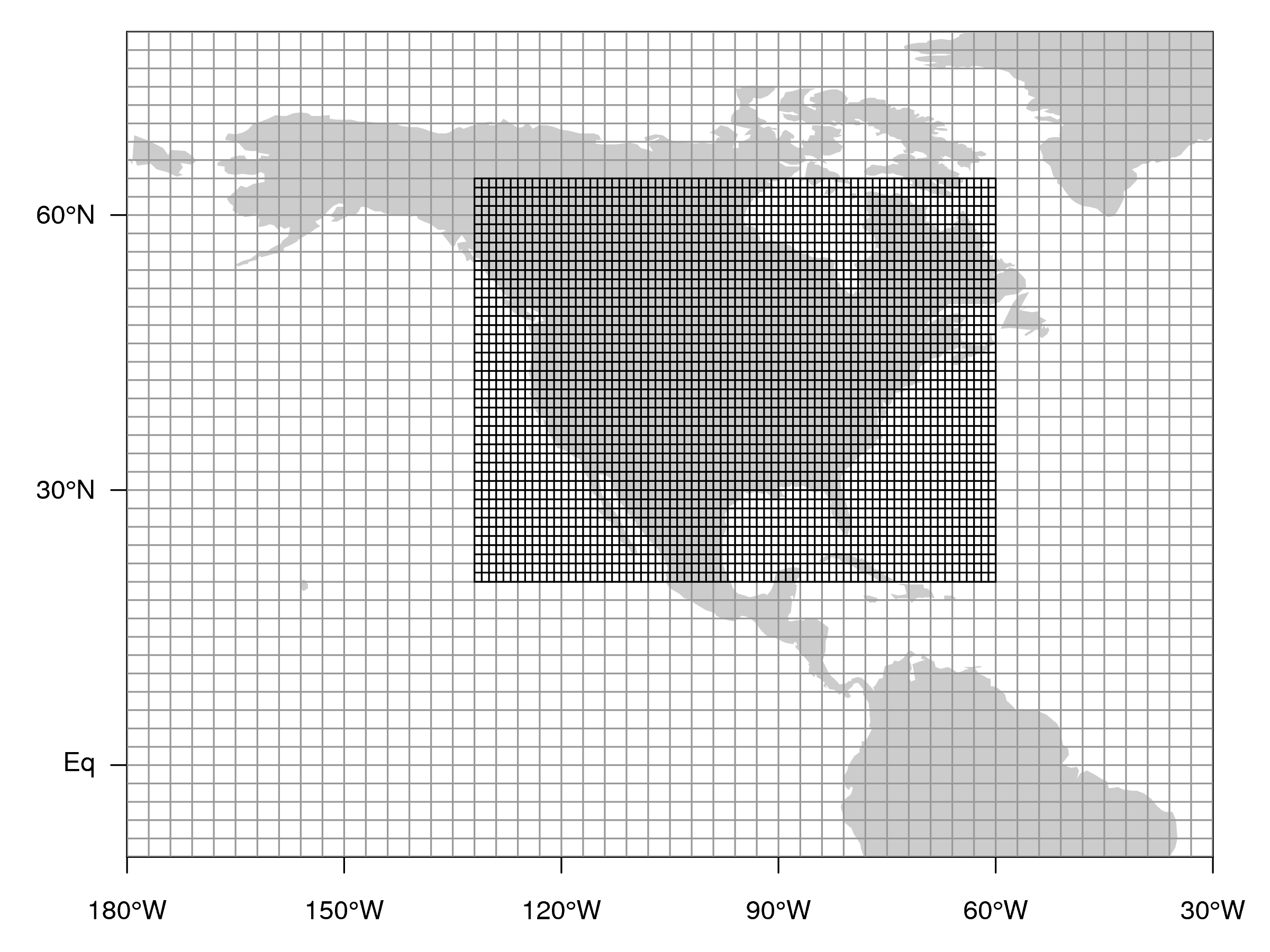
Figure 11: Nested grids used in CarbonTracker over North America. TM5 is
a global model, but it employs nested grids to provide higher
resolution over regions of interest. This figure shows the
1° × 1° nested regional grid over North America and a portion of
the global 3° lon × 2° lat grid.
The winds which drive TM5 come from two different versions of the
European Center for Medium-Range Weather
Forecasts (ECMWF) modeling system. These
two meteorological estimates are the ECMWF operational forecast model
and the ERA-interim reanalysis.
7.1.1 ECMWF operational forecast model ("od")
Operational forecasts at ECMWF are implemented using the Integrated Forecast System (IFS) model, which undergoes periodic model improvements. The IFS currently runs with 91 levels and a spectral resolution of T1279, corresponding to about 15 km horizontal resolution on a reduced Gaussian grid. The preprocessing step for TM5 reads the high-resolution forecast model results and projects them onto coarser-resolution latitude-longitude grids with resolutions varying from 6° lon × 4° lat up to 1° × 1°. TM5 uses a subset of IFS vertical layers. From the current IFS 91 layers, TM5 uses a subset of 34 layers. Prior to 2006, when the IFS used 60 vertical layers, TM5 used a 25-layer subset. Approximate heights of the mid-levels are given in Table 3.7.1.2 ERA-interim reanalysis model
The ERA-Interim reanalysis uses Cy31r2 version of the ECMWF Integrated Forecast System (IFS) model, which was used for the operational forecasts up until June 2007. That model uses a 30-minute time step and a a spectral T255 horizontal resolution, which corresponds to approximately 79 km spacing on a reduced Gaussian grid. This version of the IFS has 60 model layers in the vertical, of which TM5 uses a 25-layer subset. These levels are listed in Table 3.| "od" | "ei" | ||
| 25-layer (2000-2005) | 34-layer (2006-2012) | 25-layer | |
| 1 | 25 | 24 | 25 |
| 2 | 103 | 123 | 103 |
| 3 | 247 | 322 | 247 |
| 4 | 480 | 636 | 480 |
| 5 | 814 | 1088 | 814 |
| 6 | 1259 | 1688 | 1259 |
| 7 | 1823 | 2441 | 1822 |
| 8 | 2508 | 3349 | 2508 |
| 9 | 3318 | 4411 | 3317 |
| 10 | 4249 | 5609 | 4248 |
| 11 | 5301 | 6879 | 5300 |
| 12 | 6468 | 8151 | 6467 |
| 13 | 7741 | 9196 | 7741 |
| 14 | 9113 | 10020 | 9114 |
| 15 | 10586 | 10838 | 10588 |
| 16 | 12181 | 11651 | 12184 |
| 17 | 13925 | 12461 | 13928 |
| 18 | 15838 | 13271 | 15843 |
| 19 | 17974 | 14080 | 17983 |
| 20 | 20398 | 14889 | 20412 |
| 21 | 24410 | 15707 | 24433 |
| 22 | 29960 | 16551 | 30003 |
| 23 | 35801 | 17447 | 35895 |
| 24 | 43058 | 18423 | 43210 |
| 25 | 123496 | 19809 | 123622 |
| 26 | 21708 | ||
| 27 | 23945 | ||
| 28 | 26609 | ||
| 29 | 29826 | ||
| 30 | 33791 | ||
| 31 | 38838 | ||
| 32 | 45444 | ||
| 33 | 54047 | ||
| 34 | 129331 | ||
Table 3: Mean mid-level heights above ground in meters for the "od" 25- and 34-layer transport, and for the "ei" 25-layer transport.
7.2 Transport metrics
CT2013 is a combination of 16 independent inversions, conducted with a 4-way factorial design. As described in Sec. 8.3, we perform independent inversions for each combination of flux prior models and of transport estimate ("od" and "ei"). This results in 16 independent inversions. The results presented for CT2013 are a weighted average of these 16 inversions, where weights are assigned to the two transport models. These weights are determined by measures of transport model performance, described below. As the weights are applied only to the transport model, each of the flux priors is weighted equally in the final results.| Metric | Value | Weight | ||
| od | ei | od | ei | |
| Boundary layer height relative bias at 0 UTC | 9.0 | 9.6 | 0.5154 | 0.4846 |
| Boundary layer height relative bias at 12 UTC | 2.1 | 2.3 | 0.5249 | 0.4751 |
| SF6 interhemispheric surface bias | 0.0474 | 0.0668 | 0.5853 | 0.4147 |
| SF6 interhemispheric aircraft bias | 0.0334 | 0.0493 | 0.5964 | 0.4036 |
| Seasonal bias in northern hemisphere extratropical assimilated CO2 | 0.6448 | 0.7554 | 0.5395 | 0.4605 |
| Seasonal bias in northern hemisphere extratropical aircraft CO2 | -0.4414 | -0.5729 | 0.5648 | 0.4352 |
| MEAN | 0.5544 | 0.4456 | ||
Table 4: Summary of transport metrics used in CT2013. Each of the
individual metrics is described in following sections.
Since we treat CO2 as a passive tracer without any sources or
sinks away from the Earth's surface, simulated values of CO2 are
a linear function of surface fluxes and transport:
| (5) |
| (6) |
| (7) |
7.2.1 Boundery layer height metrics
Since CO2 has such intense and variable surface fluxes, the simulation of turbulent mixing within the planetary boundary layer (PBL) is of crucial importance for modeling atmospheric CO2. We take advantage of a recently-published dataset of PBL mixing depths diagnosed from radiosonde profiles (Seidel et al., 2012) to characterize the performance of TM5's PBL. TM5 does not use the PBL mixing depths simulated by its parent models, but instead re-diagnoses the planetary boundary layer height using a bulk Richardson scheme very similar to that of Seidel et al. (2012). As part of a Transcom model intercomparison study (Jacobson et al., 2014, in prep), the TM5 scheme was augmented to output mixing depths at the places and times of available radiosonde estimates, and with the same bulk Richardson number scheme. These simulated mixing heights were compared with thoe observed mixing heights, and results are presented in Figure 12.
Figure 12: Histograms of measured and modeled PBL depth for 0 local
solar time (left column) and 12 local solar time (right column).
Observations (green) are in the top row; "od" is shown in blue in
the middle row, and "ei" is in the bottom row.
TM5 tends to overestimate PBL depths at night
(Fig. 12, left column) whether the model is driven
by "od" or "ei" meteorology. Similarly, simulated midday mixing
depths tend to be shallower than observations (Fig. 12, right
column). However the straight magnitudes of these biases are not as
meaningful as the relative biases. This is in large part due to the
much smaller values of the mixing depth at night than during midday
hours. Thus, both BLH metrics are constructed from the ratios of the
BLH errors to the observed values.
Both "od" and "ei" have similar performance, but "od" tends to
be slightly better. The 0 LST values result in a mean relative bias
for "od" of 9.0 to the "ei" value of 9.6 and weighting of 52% and
48% respectively.
Midday model performance is similar, although the discrimination of
"od" over "ei" is slightly greater.
7.2.2 Surface SF6 metric
Sulfur hexafluoride is an industrial compound used as a dielectric in electrical equipment. Its emissions are thought to be dominated by leakage from eletrical transformers and switches. SF6 emissions are correlated both spatially and temporally with electric power usage and therefore are distributed similarly to fossil fuel CO2 emissions. It is only modestly soluble in seawater and has an estimated atmospheric lifetime of 3200 years (Ravishankara, 1993). These characterstics make SF6 an excellent tracer of large-scale atmospheric transport from northern hemisphere industrialized areas (Maiss et al., 1996). SF6 simulations were configured in TM5 by spin-up with emissions growing exponentially according to atmospheric growth rates for 1970-1990 estimated from observations. These simulations were scaled to available observations for the year 1993 from Maiss et al. (1996), and then allowed to run forward freely using EDGAR v4.2 SF6 emissions scaled to agree with observed increases in the global atmospheric burden from Levin et al. (2010). Starting in 2000, the models were sampled at the times and locations of available NOAA in situ surface observations of SF6. TM5 has historically manifested a too-great interhemispheric gradient in surface SF6 (Peters et al., 2004). The 2000-2008 mean biases (model minus observed) for each time series are plotted as a function of latitude in Figure 13 to demonstrate this transport problem. The surface SF6 metric is defined at the difference of mean 2000-2008 biases from extratropical northern hemisphere (north of 20°N) sites from those of extropical southern hemisphere (south of 20°S) sites. This metric comes out at 0.0474 ppt for "od" and 0.0668 ppt for "ei", and strongly favors "od" over "ei" transport, 59% to 41%.
Figure 13: Meridional distribution of surface SF6 bias for each observing location
7.2.3 Aircraft SF6 metric
The "od" and "ei" sulfur hexafluoride simulations described above were also sampled for available light aircraft observations of SF6. While there are fewer sites sampled by aircraft than surface instruments, the vertical distribution of these data are important for revealing atmospheric transport pathways. Little vertical structure was found in this analysis; instead, the surface interhemispheric gradient appears to be mirrored in the aircraft data. As a result, we chose a metric completely analogous to the surface SF6 metric: it is the mean of extratropical northern hemisphere residuals minus the mean of extratropical southern hemisphere residuals. For "od" this evaluates to 0.0334 ppt SF6 and for "ei", 0.0493 ppt. As a result, "od" is favored over "ei" by about 60% to 40%.7.2.4 Assimilated CO2 metric
A persistent issue with CarbonTracker performance is the existence of seasonal biases in model residuals from assimilated observations in the northern extratropics. At many sites in the northern midlatitudes, CarbonTracker manifests too much CO2 in boreal summer and too little in boreal winter. Inversion models by construction are designed to minimize all residuals for assimilated observations, and are not supposed to manifest any systematic structure in assimilated residuals. The metric we have chosen quantifies this known fault in CarbonTracker. It is the difference of mean boreal winter and mean boreal summer residuals from assimilated observations between 30°N and 60°N. Boreal summer is defined as June-September, and boreal winter is defined as November-April. The "od" transport manifests a metric value of 0.6448 ppm CO2 whereas the "ei" transport has a value of 0.7554 ppm. This results in favoring the "od" transport by about 54% to 46%.
Figure 14: Bitplot of simulated-observed residuals for assimilated
CO2 observations. Each dot represents an assimilated
observation in CT2013, and the color represents the magnitude of the
residual. In northern midlatitudes, a pronounced summertime excess
and wintertime deficit of CO2 is evident.
7.2.5 Aircraft CO2 metric
Like aircraft profiles of SF6, the vertical distribution of residuals of CO2 has the potential to reveal systematic problems with model vertical transport. While intriguing structures are evident in these aircraft profile residuals, a simple analysis suffices to reveal the most important features. As is evident in Figure 15, a summertime excess and wintertime deficit of simulated CO2 is evident throughout much of the troposphere. Aircraft data are not assimilated in CT2013, but the profiles in this metric are restricted to northern hemisphere extratropical sites. We form the difference of mean boreal winter and mean boreal summer residuals from these sites. The "od" transport has a penalty function of -0.4414 ppm CO2 and the "ei" transport a slightly worse -0.5729 ppm. This favors "od" over "ei" by 56% to 44%.
Figure 15: Posterior residuals of aircraft CO2 data, which are not
assimilated. These data, which are mostly over North America, are
grouped by latitude band and by season. The summertime excess of
CO2 is evident in both latitude bands, but is more closely
confined to the surface in the south whereas it is spread throughout
the column in the north. This is consistent with the source of the
error being localized to southern band in the summer. One potential
explanation for this is that CarbonTracker underestimates the
intensity of agricultural carbon dioxide uptake.
7.3 Further Reading
- The TM5 model homepage
- ECMWF operational forecast model (IFS) technical documentation
- ERA-interim reanalysis documentation (ECMWF)
- Peters et al., 2004, JGR paper on transport in TM5
- Krol et al., 2005, ACP overview paper of the TM5 model
- Ravishankara A.R., S. Solomon, A.A. Turnipseed, and R.F. Warren, Atmospheric lifetimes of long-lived halogenated species, Science 259,194-199,1993.
- Seidel, D. J., Y. Zhang, A. C. M. Beljaars, J.-C. Golaz, A. R. Jacobson, and B. Medeiros (2012), Climatology of the planetary boundary layer over the continental United States and Europe, J. Geophys. Res., doi:10.1029/2012JD018143
- Manfred Maiss, L.Paul Steele, Roger J. Francey, Paul J. Fraser, Ray L. Langenfelds, Neil B.A. Trivett, Ingeborg Levin, Sulfur hexafluoride—A powerful new atmospheric tracer (1996), Atmospheric Environment, Volume 30, Issues 10–11, May 1996, Pages 1621–1629
- Levin, I., Naegler, T., Heinz, R., Osusko, D., Cuevas, E., Engel, A., Ilmberger, J., Langenfelds, R. L., Neininger, B., Rohden, C. v., Steele, L. P., Weller, R., Worthy, D. E., and Zimov, S. A.: The global SF6 source inferred from long-term high precision atmospheric measurements and its comparison with emission inventories, Atmos. Chem. Phys., 10, 2655-2662, doi:10.5194/acp-10-2655-2010, 2010.
- NOAA aircraft program
- NOAA HATS group
8 Ensemble Data Assimilation
Data assimilation is the name of a process by which observations of the `state' of a system help to constrain the behavior of the system in time. An example of one of the earliest applications of data assimilation is the system in which the trajectory of a flying rocket is constantly (and rapidly) adjusted based on information of its current position, heading, speed, and other factors, to guide it to its exact final destination. Another example of data assimilation is a weather model that gets updated every few hours with measurements of temperature and other variables, to improve the accuracy of its forecast for the next day, and the next, and the next. Data assimilation is usually a cyclical process, as estimates get refined over time as more observations about the "truth" become available. Mathematically, data assimilation can be done with any number of techniques. For large systems, so-called variational and ensemble techniques have gained most popularity. Because of the size and complexity of the systems studied in most fields, data assimilation projects inevitably include supercomputers that model the known physics of a system. Success in guiding these models in time often depends strongly on the number of observations available to inform on the true system state. In CarbonTracker, the model that describes the system contains relatively simple descriptions of biospheric and oceanic CO2 exchange, as well as fossil fuel and fire emissions. In time, we alter the behavior of this model by adjusting a small set of parameters as described in the next section.8.1 Detailed Description
The four surface flux modules drive instantaneous CO2 fluxes in CarbonTracker according to:
| (8) |
8.1.1 Land-surface classification
The scaling factors λ are estimated for each week and assumed constant over this period. Each scaling factor is associated with a particular region of the global domain, and currently the geographical distribution of the regions is fixed. The choice of regions is a strong a priori constraint on the resulting fluxes and should be approached with care to avoid so-called "aggregation errors" (Kaminski et al., 2001). We chose an approach in which the ocean is divided up into 30 large basins encompassing large-scale ocean circulation features, as in the TransCom inversion study (e.g. Gurney et al., 2002). The terrestrial biosphere is divided up according to ecosystem type as well as geographical location. Thereto, each of the 11 TransCom land regions contains a maximum of 19 ecosystem types summarized in the table below. Figure 19 shows ecoregions for North America. Note that there is currently no requirement for ecoregions to be contiguous, and a single scaling factor can be applied to the same vegetation type on both sides of a continent. Further details on ecoregions can be found in the ecoregions docuementation section. Theoretically, this approach leads to a total number of 11*19+30=239 optimizable scaling factors λ each week, but the actual number is 156 since not every ecosystem type is represented in each TransCom region, and because we decided not to optimize parameters for ice-covered regions, inland water bodies, and desert. The total flux coming out of these last regions is negligibly small. It is important to note that even though only one parameter is available to scale, for instance, the flux from coniferous forests in Boreal North America, each 1° × 1° grid box predominantly covered by coniferous forests will have a different flux F(x,y,t) depending on local temperature, radiation, and CASA modeled monthly mean flux. Ecosystem types considered on 1° × 1° for the terrestrial flux inversions is based on Olson, (1992). Note that we have adjusted the original 29 categories into only 19 regions. This was done mainly to fill the unused categories 16, 17, and 18, and to group the similar (from our perspective) categories 23-26+29. Table 5 shows each vegetation category considered. Percentages indicate the area associated with each category for North America rounded to one decimal.| category | Olson V 1.3 | Percentage area |
| 1 | Conifer Forest | 19.0% |
| 2 | Broadleaf Forest | 1.3% |
| 3 | Mixed Forest | 7.5% |
| 4 | Grass/Shrub | 12.6% |
| 5 | Tropical Forest | 0.3% |
| 6 | Scrub/Woods | 2.1% |
| 7 | Semitundra | 19.4% |
| 8 | Fields/Woods/Savanna | 4.9% |
| 9 | Northern Taiga | 8.1% |
| 10 | Forest/Field | 6.3% |
| 11 | Wetland | 1.7% |
| 12 | Deserts | 0.1% |
| 13 | Shrub/Tree/Suc | 0.1% |
| 14 | Crops | 9.7% |
| 15 | Conifer Snowy/Coastal | 0.4% |
| 16 | Wooded tundra | 1.7% |
| 17 | Mangrove | 0.0% |
| 18 | Non-optimized areas (ice, polar desert, inland seas) | 0.0% |
| 19 | Water | 4.9% |
Table 5: Ecosystem types over North America
Each 1° × 1° pixel of our domain was assigned one of the categories
above based on the Olson category that was most prevalent in the 0.5°×0.5° underlying area.
8.1.2 Ensemble Size and Localization
The ensemble system used to solve for the scalar multiplication factors is similar to that in Peters et al. (2005) and based on the square root ensemble Kalman filter of Whitaker and Hamill, (2002). We have restricted the length of the smoother window to only five weeks as we found the derived flux patterns within North America to be robustly resolved well within that time. We caution the CarbonTracker users that although the North American flux results were found to be robust after five weeks, regions of the world with less dense observational coverage (the tropics, Southern Hemisphere, and parts of Asia) are likely to be poorly observable even after more than a month of transport and therefore less robustly resolved. Although longer assimilation windows, or long prior covariance length-scales, could potentially help to constrain larger scale emission totals from such areas, we focus our analysis here on a region more directly constrained by real atmospheric observations. Ensemble statistics are created from 150 ensemble members, each with its own background CO2 concentration field to represent the time history (and thus covariances) of the filter. To dampen spurious noise due to the approximation of the covariance matrix, we apply localization (Houtekamer and Mitchell, 1998) for non-MBL sites only. This ensures that tall-tower observations within North America do not inform on for instance tropical African fluxes, unless a very robust signal is found. In contrast, MBL sites with a known large footprint and strong capacity to see integrated flux signals are not localized. Localization is based on the linear correlation coefficient between the 150 parameter deviations and 150 observation deviations for each parameter. If the relationship between a parameter deviation and its modeled observational impact is statistically significant, then that relationship is used to modify parameters. Otherwise, the relationship is assumed to be spurious noise due to the numerical approximation of the covariance matrix by the limited ensemble. We accept relationships that reach 95% significance in a student's T-test with a two-tailed probability distribution.8.1.3 Dynamical Model
In CarbonTracker, the dynamical model is applied to the mean parameter values λ as:
| (9) |
8.2 Covariance Structure
The prior covariance structure P−0 describes the magnitude of the uncertainty on each parameter, plus their correlation in space. The latter is applied such that correlations between the same ecosystem types in different TransCom regions decrease exponentially with distance (L=2000km), and thus assumes a coupling between the behavior of the same ecosystems in close proximity to one another (such as coniferous forests in Boreal and Temperate North America). Furthermore, all ecosystems within tropical TransCom regions are coupled decreasing exponentially with distance since we do not believe the current observing network can constrain tropical fluxes on sub-continental scales, and want to prevent spurious compensating source/sink pairs ("dipoles") to occur in the tropics. In our standard assimilation, the chosen standard deviation is 80% on land parameters. All parameters have the same variance within the land or ocean domain. Because the parameters multiply the net-flux though, ecosystems with larger weekly mean net fluxes have a larger variance in absolute flux magnitude.8.3 Multiple prior models
In Bayesian estimation systems like CarbonTracker, there is a potential for bias from a flux prior to propagate through the inversion system to the final result. It is difficult to quantify this effect, and as a result it is generally considered a requirement that flux priors be unbiased. We cannot guarantee this for any of our prior fluxes, be they the prior estimates for terrestrial or oceanic exchange, or the presumed wildfire and fossil fuel emissions. In order to explicitly quantify the impact of prior bias on our solution, in CT2013 we present the result of a multi-model prior suite of inversions. We have used two terrestrial flux priors, two air-sea exchange priors, and two estimates of imposed fossil fuel emissions in a factorial design experiment. For each of the resulting eight unique combinations of prior fluxes, we conduct an independent inversion conducted independently according to the methods described above. We present as a final result the mean flux across this suite of inversions and the atmospheric CO2 distribution resulting from applying these mean fluxes to our atmospheric transport model. Each of the priors is described in detail in its corresponding documentation section. Furthermore, with CT2013 we introduce the use of multiple atmospheric transport estimates. As described in section 7, we perform the eight-way inversion suite for each of the two transport estimates, then combine the mole fraction and flux results using a weighted average. The weights are assigned to each of the transport estimates based on metrics which quantify the transport model performance. See 7.2 for details.
Figure 16: CT2013 prior covariance structure. The prior
covariance matrix (top panel) and the square root of diagonal members of
this matrix (bottom panel). Covariance matrix quantities are
dimensionless squared scaling factors, and the bottom panel is the
square root of this. TransCom land
regions form the first 11 large divisions on the axes here. As
described above, each of those regions contains 19 potential ecosystems.
Correlations between similar ecosystems in proximate Transcom regions
are visible in North America (e.g. NABR and NATM, the boreal and
temperate North American regions) and Eurasia. Within tropical Transcom
regions, however, differing ecosystems are assigned a non-zero prior
covariance, which is visible here as red block-like structures on the
diagonal within, for example, the South America Tropical (SATR) Transcom
region. Ocean regions have a more complicated covariance structure that
depends on which prior is used; the structure shown here is that of the
ocean inversion flux prior. The
lower panel of this diagram compares the on-diagonal elements of the
prior covariance matrix by plotting their square roots. The resulting
standard deviations are directly comparable to the percentages discussed
in section 3 above; 0.8 is equivalent to 80%. The retuning of the
covariance matrix for CT2013's multiple-prior simulation is made
evident by also showing these values from previous CarbonTracker
releases in red.
8.3.1 Posterior Uncertainties in CarbonTracker
The formal "internal" error estimates produced by CarbonTracker are unrealistically large. This is largely a result of the relatively short assimilation window in CarbonTracker, along with a dynamical model that introduces a fresh prior covariance matrix with every new week entering the assimilation window. This five-week window effectively inhibits the formation of anticorrelations ("dipoles") in flux estimates, and does little to reduce the confidence interval on prior fluxes. The temporal truncation in CarbonTracker imposed by its five-week assimilation window tends to yield regional flux estimates that are largely uncorrelated with those from other regions. A consequence of this feature is that uncertainties in CarbonTracker tend to increase as larger regions are considered; regional errors mostly just add in quadrature without any cancellation from dipole anticorrelation. Whereas many inversions yield smaller errors as the spatial extent of the region being considered increases, CarbonTracker acts in the opposite fashion. This is perhaps most obvious in the estimate of CarbonTracker's global annual surface flux of carbon dioxide. While CT2013 estimates a one-sigma error of more than 6 PgC yr−1 on its global flux, this quantity is in actuality much more well-constrained. This is evident from CarbonTracker's excellent agreement with observational estimates of atmospheric growth rate. In CT2013, error estimates are about a factor of two larger than in previous releases, mainly due to the retuning of the land prior covariance discussed above. However, uncertainties presented for CT2013 take into account not only the "internal" flux uncertainty generated by a single inversion, but also the across-model "external" uncertainty representing the spread of the inversion models due to the choice of prior flux.8.4 Further Reading
- Whitaker and Hamill, 2002 paper
- Peters et al., 2005 paper
- Olson ecosystem types, data
- Kaminski et al., Journal of Geophysical Research, Vol. 106, No. D5, PP. 4703-4715, 2001 doi:10.1029/2000JD900581
9 Ecoregions in CarbonTracker
9.1 What are ecoregions?
Ecoregions are the actual scale on which CarbonTracker performs its optimization over the land. Ecoregions are meant to represent large expanses of land within a given continent having similar ecosystem types, and are used to divide continents into smaller pieces for analysis. The ecosystem types use in CarbonTracker are derived from the Olson (1992) vegetation classification (Table 6, Figure 17). We define an ecoregion as an ecosystem type within a given Transcom land region. There are 11 such Transcom land regions (Figure 18), so there are 11*19 = 209 possible ecoregions. However, not all ecosystem types are present in all Transcom regions, and the actual number of land ecoregions ends up being 126. Note on "Semitundra": this is a potentially misleading shorthand abbreviation for a collection of ecosystems comprising semi-desert, shrubs, steppe, and polar+alpine tundra. The "Semitundra" zones appearing in northern Africa where one expects to find the Sahara desert are not, of course, tundra environments. They are instead semi-desert zones.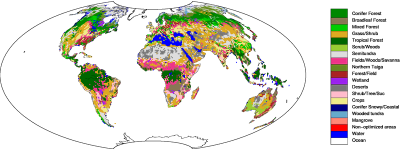
Figure 17: Global distribution of Olson ecosystem types.
| Ecosystem Type | North American Boreal | North American Temperate | ||
| Area (km2) | Percentage | Area (km2) | Percentage | |
| Conifer Forest | 2315376 | 22.9% | 1607291 | 14.0% |
| Broadleaf Forest | - | - | 269838 | 2.4% |
| Mixed Forest | 592291 | 5.9% | 930813 | 8.1% |
| Grass/Shrub | 53082 | 0.5% | 2515582 | 21.9% |
| Tropical Forest | - | - | 58401 | 0.5% |
| Scrub/Woods | - | - | 416520 | 3.6% |
| Semitundra | 3396292 | 33.6% | 866468 | 7.6% |
| Fields/Woods/Savanna | 29243 | 0.3% | 1020939 | 8.9% |
| Northern Taiga | 1658773 | 16.4% | - | - |
| Forest/Field | 61882 | 0.6% | 1243174 | 10.8% |
| Wetland | 322485 | 3.2% | 66968 | 0.6% |
| Deserts | - | - | 21934 | 0.2% |
| Shrub/Tree/Suc | - | - | 11339 | 0.1% |
| Crops | - | - | 1969912 | 17.2% |
| Conifer Snowy/Coastal | 41440 | 0.4% | 73437 | 0.6% |
| Wooded tundra | 360388 | 3.6% | 6643 | 0.1% |
| Mangrove | - | - | - | - |
| Non-optimized areas | - | - | - | - |
| Water | 1269485 | 12.6% | 384728 | 3.4% |
| Total | 10100736 | 100.0% | 11463986 | 100.0% |
Table 6: Ecosystem areas over the two Transcom regions covering North America.
9.2 Why use ecoregions?
A fundamental challenge to atmospheric inversions like CarbonTracker is that there are not enough observations to directly constrain fluxes at all times and in all places. It is therefore necessary to find a way to reduce the number of unknowns being estimated. Strategies to reduce the number of unknowns in problems like this one generally impose information from external sources. In CarbonTracker, we reduce the problem size both by estimating fluxes at the ecoregion scale, and by using a terrestrial biological model to give a first guess flux from the ecoregion. The model is also used to give the spatial and temporal distribution of CO2 flux within a region and week.9.3 Ecosystems within Transcom regions
Each Transcom land region (Figure 18) can contain up to 19 ecoregions.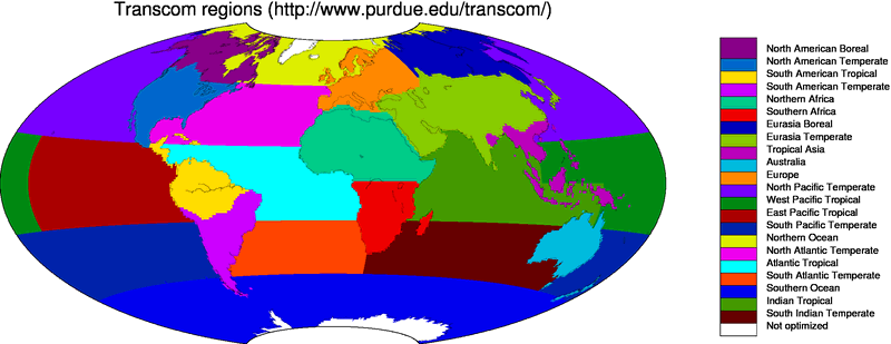
Figure 18: The 11 land regions and 11 ocean regions of the Transcom project
.
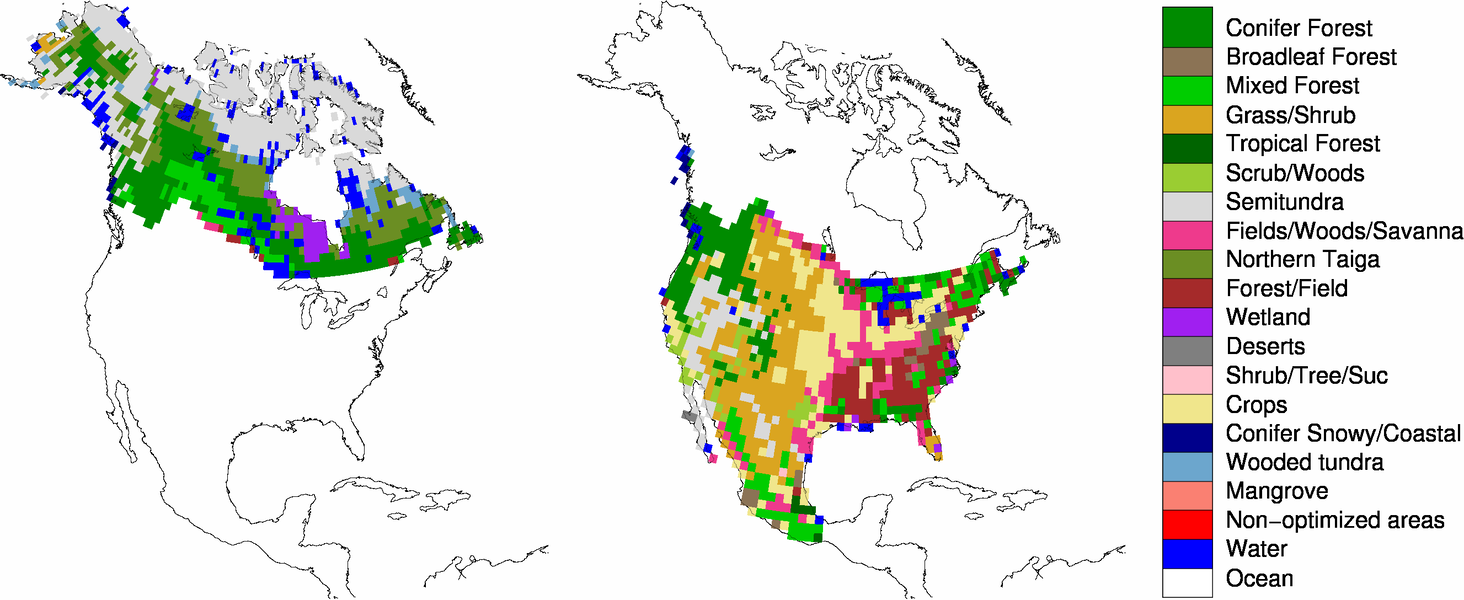
Figure 19: Ecoregions within the North American Boreal (left)
and North American Temperate (right) Transcom regions.
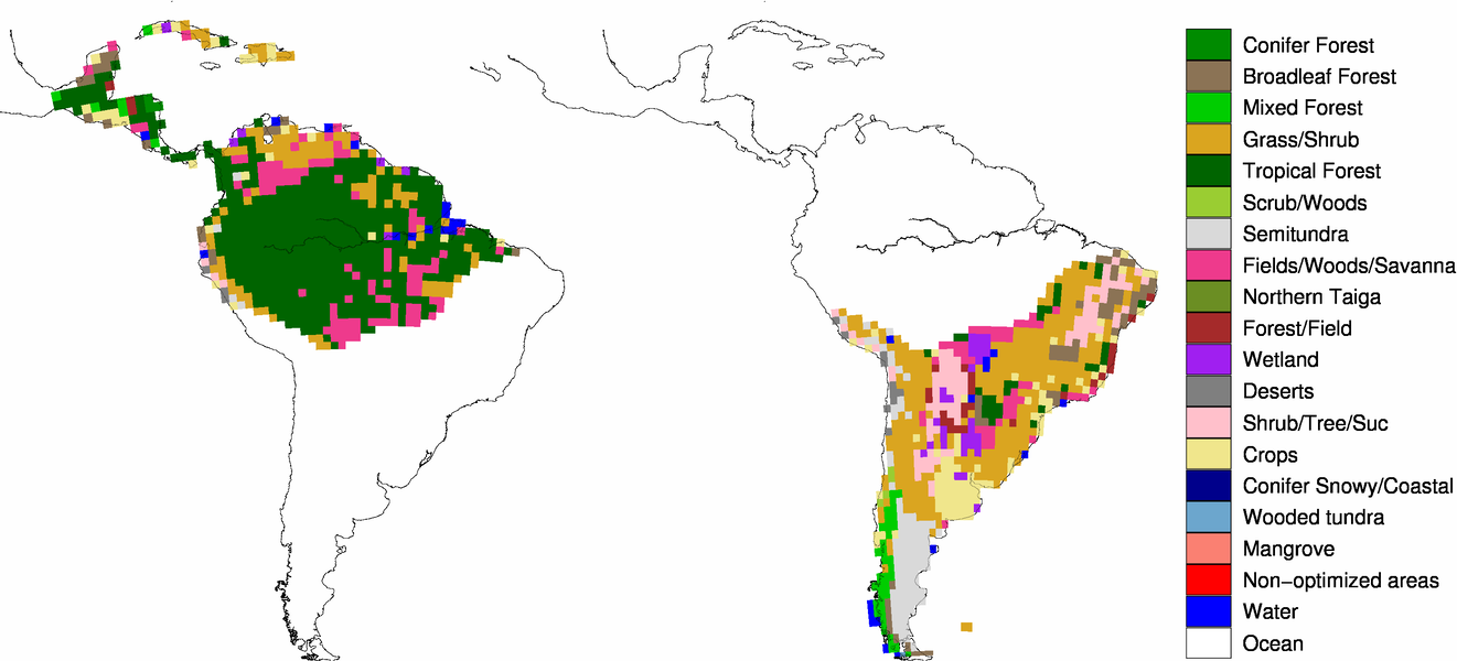
Figure 20: Ecoregions within the South American Tropical (left)
and South American Temperate (right) Transcom regions.
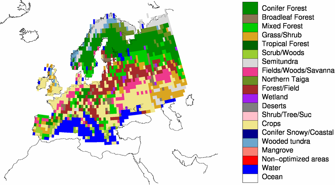
Figure 21: Ecoregions within the Europe Transcom region.
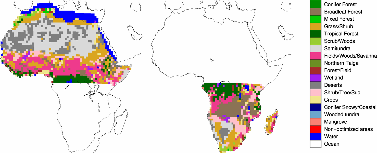
Figure 22: Ecoregions within the Northern Africa (left) and
Southern Africa (right) Transcom regions.
9.4 Further Reading
File translated from TEX by TTH, version 4.04.
On 14 Nov 2014, 12:07.