1. Introduction
The oceans play an important role in the Earth's carbon cycle. They
are the largest long-term sink for carbon and have an enormous
capacity to store and redistribute CO2 within
the Earth system.
Oceanographers estimate that about 48% of the CO2 from fossil fuel burning has been absorbed by the
ocean [Sabine et al., 2004]. The dissolution of CO2 in seawater shifts the balance of the ocean
carbonate equilibrium towards a more acidic state with a lower
pH. This effect is already measurable [Caldeira and Wickett, 2003],
and is expected to become an acute challenge to shell-forming
organisms over the coming decades and centuries.
Although the oceans as a whole have been a relatively steady net
carbon sink, CO2 can also be released from
oceans depending on local temperatures, biological activity, wind
speeds, and ocean circulation.
These processes are all considered in CarbonTracker, since they can
have significant effects on the ocean sink.
Improved estimates of the air-sea exchange of carbon in turn help us
to understand variability of both the atmospheric burden of CO2 and terrestrial carbon exchange.
|
|
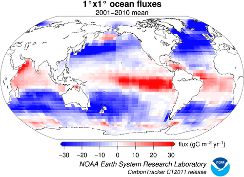
Figure 1. Posterior long-term mean ocean fluxes from CarbonTracker. The pattern of air-sea exchange of
CO2 averaged over the time period indicated,
as estimated by CarbonTracker. Negative fluxes
(blue colors) represent CO2 uptake by the
ocean, whereas positive fluxes (red colors) indicate regions in which
the ocean is a net source of CO2 to the
atmosphere. Units are gC m-2 yr-1.
|
The initial release of CarbonTracker (2007) used climatogical
estimates of CO
2 partial pressure in surface
waters (pCO
2) from Takahashi et al. [2002] to compute a first-guess air-sea
flux. This air-sea pCO
2 disequilibrium was
modulated by a surface barometric pressure correction before being
multiplied by a gas-transfer coefficient to yield a flux. Starting
with CarbonTracker 2007B and continuing through the CT2010 release,
the air-sea pCO
2 disequilibrium was imposed
from analysis of ocean inversions ("OIF", cf. Jacobson et al., 2007)
results, with short-term flux variability derived from the atmospheric
model wind speeds via the gas transfer coefficient. The barometric
pressure correction was removed so that climatological high- and
low-pressure cells did not bias the long-term means of the first guess
fluxes.
Starting with the CT2011 release, two models are used to provide prior
estimates of air-sea CO2 flux. The OIF
scheme provides one of these flux priors, and the other is an updated
version of the Takahashi et al. pCO2
climatology.
2. Detailed Description
Oceanic uptake of CO2 in CarbonTracker is
computed using air-sea differences in partial pressure of CO2 inferred either from ocean inversions (called
"OIF" henceforth), or from a compilation of direct measurements of
seawater pCO2 (called "pCO2-clim" henceforth).
These air-sea partial pressure differences are combined with a gas
transfer velocity computed from wind speeds in the atmospheric
transport model to compute fluxes of carbon dioxide across the sea surface.
In either method, the first-guess fluxes have no interannual
variability (IAV) other than a smooth trend. IAV in oceanic CO2 flux is due to anomalies in surface pCO2, such as those that occur in the tropical eastern
Pacific during an El Niño, and to associated variability in
winds, ocean circulation, and sea-surface properties. In
CarbonTracker, only the surface winds (and hence gas transfer),
manifest these interannual anomalies; the remaining IAV of flux must
be inferred from atmospheric CO2 signals.
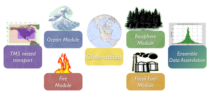
In the following sections we describe the two ocean flux prior
models. We then describe the air-sea gas transfer velocity
parameterization and discuss detais of the inversion methodology
specific to oceanic exchange of CO2. Figures
comparing the air-sea flux priors are presented in Box 1 below.
2.1 OIF: the Ocean Inversion Fluxes prior
For the OIF prior, long-term mean air-sea fluxes and the
uncertainties associated with them are derived from the ocean interior
inversions reported in Jacobson et al. [2007]. These ocean inversion
flux estimates are composed of separate preindustrial (natural)
and anthropogenic flux inversions based on the methods described in
Gloor et al. [2003] and biogeochemical interpretations of Gruber,
Sarmiento, and Stocker [1996]. The uptake of anthropogenic CO2 by the ocean is assumed to increase in proportion
to atmospheric CO2 levels, consistent with
estimates from ocean carbon models.
OIF contemporary pCO2 fields were computed by
summing the preindustrial and anthropogenic flux components from
inversions using five different configurations of the Princeton/GFDL
MOM3 ocean general circulation model [Pacanowski and Gnanadesikan,
1998], then dividing by a gas transfer velocity computed from the
European Centre for Medium-Range Weather Forecasts (ECMWF) ERA40
reanalysis. There are two small differences in first-guess fluxes in
this computation from those reported in Jacobson et al. [2007].
First, the five OIF estimates all used Takahashi et al. [2002]
pCO2 estimates to provide high-resolution
patterning of flux within inversion regions (the alternative "forward"
model patterns were not used). To good approximation, this choice
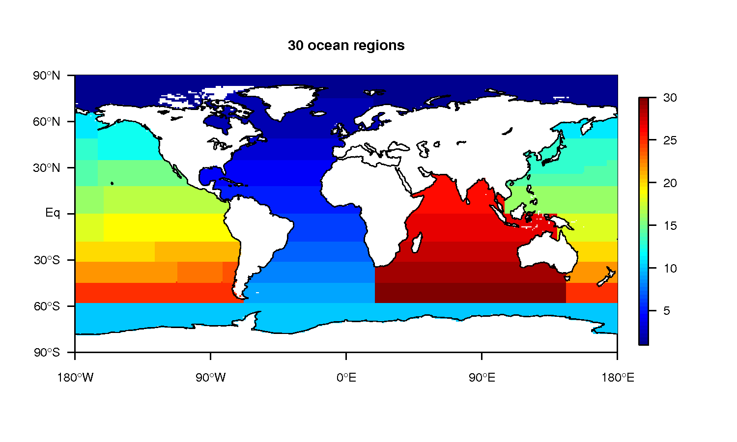
only affects the spatial and temporal distribution of flux within each
of the 30 ocean inversion
regions, not the magnitude of the estimated flux. Second, wind
speed differences between the ERA40 product used in the offline
analysis and the ECMWF operational model used in the online
CarbonTracker analysis result in small deviations from the OIF
estimates.
Other than the smooth trend in anthropogenic flux assumed
by the OIF results, interannual variability (IAV) in the first guess
ocean flux comes entirely from wind speed effects on the gas transfer
velocity. This is because the ocean inversions retrieve only a
long-term mean and smooth trend.
2.2 pCO2-Clim: Takahashi et al. [2009] climatology prior
The pCO2-Clim prior is derived from the
Takahashi et al. [2009] climatology of seawater pCO2. This climatology was created from about 3
million direct observations of seawater pCO2
around the world between 1970 and 2007. With the exception of
measurements in the Bering Sea, these observations were all linearly
extrapolated to the corresponding month of the year 2000 by assuming a
constant trend of 1.5 μatm yr-1. This set
of global monthly measurements corrected to the reference year 2000
was then interpolated onto a regular grid using a modeled surface
current field.
The Takahashi et al. [2009] product goes beyond providing this
estimate of surface water pCO2. They also
compute climatological air-sea exchange of CO2 by using the GLOBALVIEW-CO2 atmospheric carbon dioxide product to infer
air-sea ΔpCO2, sea surface properties
inferred from ocean climatologies, and winds from atmospheric
reanalysis to estimate gas-transfer velocity. Unlike other
atmospheric analyses, we have chosen not to use the climatological
fluxes as our prior, nor to use the climatological ΔpCO2. Instead, we take only the seawater pCO2 distribution from the Takahashi et
al. climatology--our atmospheric model provides both pCO2 in the air at the sea surface and the winds
needed to estimate gas transfer. Seawater pCO2 is extrapolated from 2000 to the actual year of
the CarbonTracker simulation using the presumed increase of 1.5
μatm yr-1 at every point in the global
ocean.
2.3 Gas-transfer velocity and ocean surface properties
Both priors use CO2 solubilities and Schmidt
numbers computed from World Ocean Atlas 2009 (WOA09) climatological
fields of sea surface temperature [Locarnini et al., 2010] and sea
surface salinity [Antonov et al., 2010] fields. Gas transfer velocity
in CarbonTracker is parameterized as a quadratic function of wind
speed following Wanninkhof [1992], using the formulation for
instantaneous winds. Gas exchange is computed every 3 hours using
wind speeds from the ECMWF operational model as represented by the TM5 atmospheric transport
model.
Air-sea transfer is inhibited by the presence of sea ice, and for this
work fluxes are scaled by the daily sea ice fraction in each gridbox
provided by the ECMWF forecast data.
Box 1. Comparison of air-sea flux priors
|
|
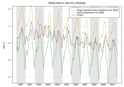
Time series of global-total ocean flux among the two priors and the
CT2011 posterior. Global CO2
uptake by the ocean, expressed in PgC yr-1.
Positive flux represents a gain of CO2 to the atmosphere,
and the negative numbers here indicate that the ocean is a sink of
CO2. While both priors manifest similar trends of
increasing oceanic uptake of CO2, the OIF prior (in green)
has more oceanic uptake and a greater annual cycle than the
pCO2-clim prior (in tan).
The CT2011 across-model posterior estimate is shown in black for comparison.
|
|
|
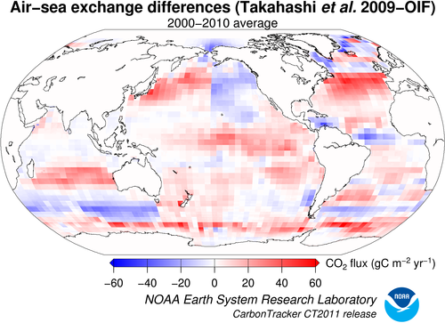
Differences in long-term mean
ocean fluxes between the two priors. Red indicates areas where the
pCO2-clim prior has less oceanic uptake (or
more outgassing to the atmosphere) than the OIF prior, and blue
represents the opposite. Units are gC m-2
yr-1.
|
2.4. Specifics of the Inversion Methodology Specific to Air-sea CO2 Fluxes
The first-guess fluxes described here are subject to scaling during
the CarbonTracker optimization process, in which atmospheric CO2 mole fraction observations are combined with
transport simulated by the atmospheric model to infer flux signals.
Prior air-sea fluxes are adjusted within each of of the 30 ocean inversion regions. In
this process, signals of terrestrial flux in atmospheric CO2 distribution can be erroneously interpreted as
being caused by oceanic fluxes. This flux "aliasing" or "leakage" is
evident in some regions as a change in the shape of the seasonal cycle
of air-sea flux.
Prior uncertainties for the OIF and pCO2-clim
models are specified as uncertainties on scaling factors multiplying
net CO2 flux in each of the 30 ocean inversion regions. The
pCO2-clim prior has independent regional
uncertainties (a diagonal prior covariance matrix), with the
uncertainty standard deviation on each region set to 40%. The OIF
prior uncertainty has a fully-covariate covariance matrix with
off-diagonal elements representing the results of the ocean inversion
of Jacobson et al. [2007]. The pre-industrial flux uncertainty is
time-indepedendent, but the anthropogenic flux uncertainty grows in
time as anthropogenic flux uptake increases. The latter is scaled to
the simulation date, then added to the former. Total uncertainties
are consistent with the Jacobson et al. [2007] results.
3. Further Reading
- NOAA Pacific Marine Environmental Laboratory (PMEL)
- Ocean Acidification
- Antonov, J. I., D. Seidov, T. P. Boyer, R. A. Locarnini, A. V. Mishonov, H. E. Garcia, O. K. Baranova, M. M. Zweng, and D. R. Johnson, 2010. World Ocean Atlas 2009, Volume 2: Salinity. S. Levitus, Ed. NOAA Atlas NESDIS 69, U.S. Government Printing Office, Washington, D.C., 184 pp.
- Caldeira, K., and M. E. Wickett (2003), Anthropogenic carbon and ocean pH, Nature, 425365-365.
- GLOBALVIEW-CO2: Cooperative Atmospheric Data Integration Project - Carbon Dioxide. CD-ROM, NOAA ESRL, Boulder, Colorado [Also available on Internet via anonymous FTP to ftp.cmdl.noaa.gov, Path: ccg/co2/GLOBALVIEW], 2011.
- Gloor, M., N. Gruber, J. Sarmiento, C. L. Sabine, R. A. Feely, and C. Rödenbeck (2003), A first estimate of present and preindustrial air-sea CO2 flux patterns based on ocean interior carbon measurements and models, Geophysical Research Letters, 30, 10.1029/2002GL015594.
- Gruber, N., J. L. Sarmiento, and T. F. Stocker (1996), An improved method for detecting anthropogenic CO2 in the oceans, Global Biogeochemical Cycles, 10, , 809-837.
- Jacobson, A. R., N. Gruber, J. L. Sarmiento, M. Gloor, and S. E. Mikaloff Fletcher (2007), A joint atmosphere-ocean inversion for surface fluxes of carbon dioxide: I. Methods and global-scale fluxes, Global Biogeochemical Cycles, 21, doi:10.1029/2005GB002556.
- Locarnini, R. A., A. V. Mishonov, J. I. Antonov, T. P. Boyer, H. E. Garcia, O. K. Baranova, M. M. Zweng, and D. R. Johnson, 2010. World Ocean Atlas 2009, Volume 1: Temperature. S. Levitus, Ed. NOAA Atlas NESDIS 68, U.S. Government Printing Office, Washington, D.C., 184 pp.
- Pacanowski, R. C., and A. Gnanadesikan (1998), Transient response in a z-level ocean model that resolves topography with partial cells, Monthly Weather Review, 126, 3248--3270.
- Sabine, C. L., R. A. Feely, N. Gruber, R. M. Key, K. Lee, J. L. Bullister, R. Wanninkhof, C. S. Wong, D. W. R. Wallace, B. Tilbrook, F. J. Millero, T. H. Peng, A. Kozyr, T. Ono, and A. F. Rios (2004), The oceanic sink for anthropogenic CO2, Science, 305, 367-371.
- Takahashi, T., S. C. Sutherland, C. Sweeney, A. P. N. Metzl, B. Tilbrook, N. Bates, R. Wanninkhof, R. A. Feely, C. Sabine, J. Olafsson, and Y. Nojiri (2002), Global air-sea CO2 flux based on climatological surface ocean pCO2, and seasonal biological and temperature effects, Deep-Sea Research II, 49, 1601--1622.
- Takahashi, T., S. C. Sutherland, C. Sweeney, R. A. Feely, D. W. Chipman, B. Hales, G. Friederich, F. Chavez, C. Sabine, A. Watson, D. C. E. Bakker, U. Schuster, N. Metzl, H. Yoshikawa-Inoue, M. Ishii, T. Midorikawa, Y. Nojiri, A. Kortzinger, T. Steinhoff, M. Hoppema, J. Olaffson, T. S. Anarson, B. Tilbrook, T. Johannessen, A. Olsen, R. Bellerby, C. S. Wong, B. Delille, N. R. Bates, and H. J. W. de Baar (2009), Climatological mean and decadal change in surface ocean pCO2, and net sea-air CO2 flux over the global oceans, Deep-Sea Resarch II, 56, 554--577.
- Wanninkhof, R. (1992), Relationship between wind speed and gas exchange over the ocean, Journal of Geophysical Research, 97, 7373--7382.
