• Home
• PSL Home
• Climate Data and Resources
• HRC Atlas

Contents

PRELIMINARIES

Acknowledgments

Introduction

Data Sources

Analysis Procedures

Cautionary Notes

Effects of the 24-hour cycle of convection

Consequences of subjective interpretation of data

The average density of HRC

The "edge" effect

References

MAPS

Part I. Location and Frequency of Highly Reflective Clouds: Means of Monthly Data

Part II. Coefficients of Variation of the Number of Days With Highly Reflective Clouds for Each Month

Part III. Location and Frequency of Highly Reflective Clouds: Normalized Monthly Data

---

Acknowledgments

Funding for the HRC project has been provided since 1979 by the Equatorial Pacific Ocean Climate Studies (EPOCS) program of NOAA's Environmental Research Laboratories. Initial work on the project was conducted at the joint Institute for Marine and Atmospheric Research (NOAA-University of Hawaii) in Honolulu. Since 1981, HRC data have been gathered at the Cooperative Institute for Research in the Environmental Sciences (NOAA-University of Colorado) in Boulder.

Many people have contributed to this project. Special thanks are due to Colin Ramage of the University of Hawaii and Joseph Fletcher of NOAA for their support, guidance, and encouragement. Bernard Kilonsky, Steven Thomas, Steven Lyons, S. J. S. Khalsa, and Arnold Hori were instrumental in setting up and streamlining the original data extraction procedures at the University of Hawaii. The author also thanks his colleagues in the Climate Research Program, especially George Kiladis, Richard Keen, Henry Diaz, and Robert Grossman for their helpful comments and critical evaluations of the HRC data set.

At the University of Colorado, Vincent Troisi was responsible for writing and implementing the digitizing and data storage and retrieval procedures. Mark Anderson, John Watkins, and Robert Crane spent countless hours analyzing thousands of satellite picture mosaics. Stuart Naegele was invaluable in helping organize and improve the quality of the material presented. Of great importance was the contribution of the digitizers: Michael Roberts, Elizabeth Bridges, Stacy Michaels, John Rife, and John Harbor. Their patience and perseverance are greatly appreciated. Joseph Thorn assisted in preparing material for publication. Editorial Services of the Environmental Research Laboratories in Boulder provided editing and design, and coordinated production of the Atlas.

---

Introduction

More than 25 years have passed since the first meteorological satellite, TIROS-1, was launched. Among the many benefits of the satellite era in meteorology has been the development of a record of satellite images covering the entire tropical belt, including the oceans and other remote areas not accessible by previous methods of observation. The record is now sufficiently extensive to have value for climatological work.

The polar-orbiting satellites operated by the National Oceanic and Atmospheric Administration (NOAA) record images over a strip approximately 15 longitudinal degrees wide. Because the satellites are placed in sun-synchronous orbits, specific points in the global tropics are sampled twice a day, 12 hours apart, at approximately the same local times every day. However, these local times have changed over the period of record as a result of changes in the orbital parameters of the satellites.

In 1970, NOAA began producing computer-generated mosaics of these satellite images, using Mercator projections (Conlan, 1973). The mosaics contain a wealth of information on cloud conditions around the global tropics. Unfortunately, the quality of the mosaics has varied considerably with respect to background brightness, resolution, and contrast. Even individual mosaics show significant changes in brightness levels, such as those apparent within individual orbit passes in the mosaic shown in Figure 1; therefore, they must be carefully interpreted. Any summary of cloud information from the mosaics for a specific period of time, using a simple, objective criterion such as the mean brightness level, will contain many errors.

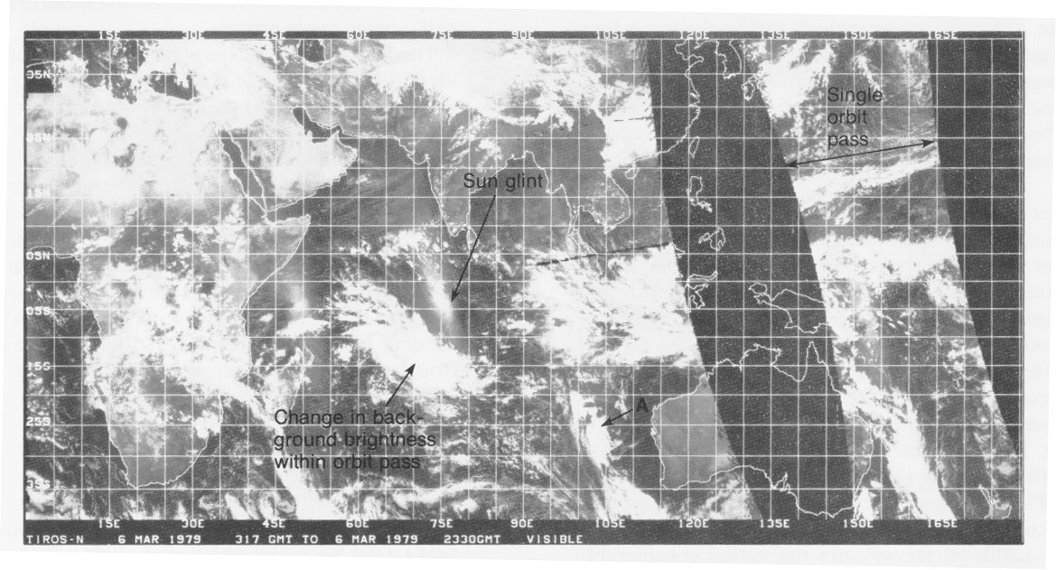
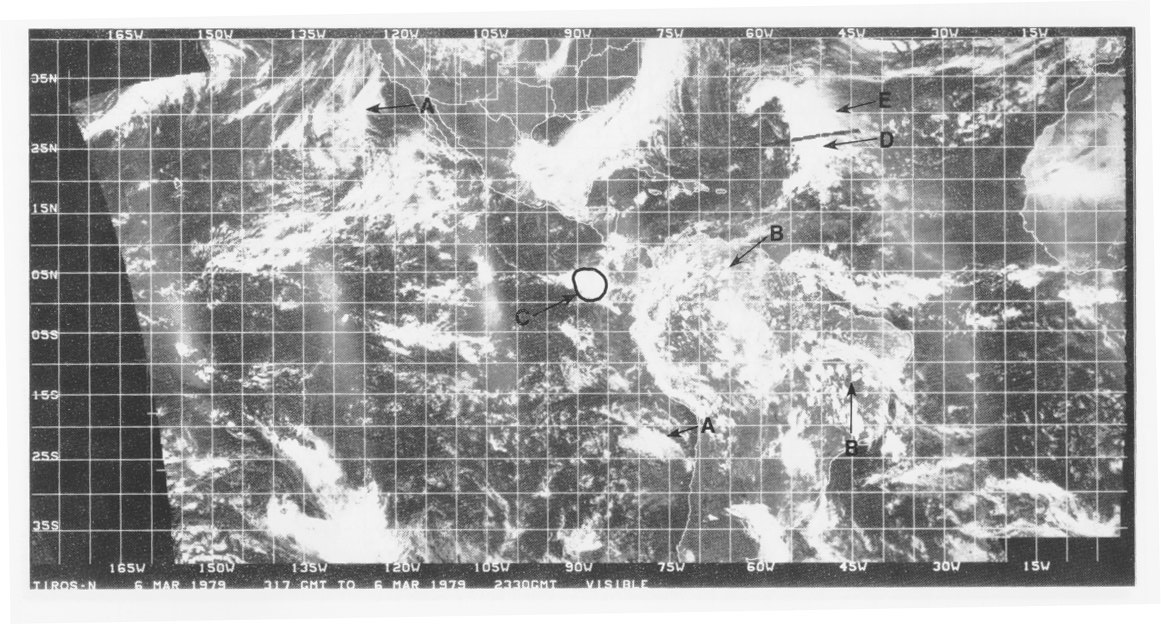
Figure 1. Sample Mercator projection mosaics composed of visible-range imagery obtained from NOAA's TIROS-N polar-orbiting satellite on 6 March 1979. The width of one orbit pass in indicated. Swaths of missing data are evident, as are changes in background brightness within a single orbit pass. Satellite pass time for points along the Equator is approximately 1530 LT. Samples of the following cloud types are identified: (A) stratus; (B) cumulonimbus (small convective clouds); (C) cumulonimbus (HRCs); (D) thick cirrostratus; (E) thin cirrostratus. Sunglint is the sun's reflection on unclouded ocean surface.

The data presented here are the record of subjectively identified areas of large-scale organized convection over the global tropics on the daily daytime Mercator projection mosaics for a 15-year period from 1971 to 1985. These convection areas appear as highly reflective clouds in the visible-range mosaics and as white areas in the infrared (IR) range. Highly reflective cloud (HRC) is defined here as a deep, organized tropical convection system extending at least 200 km horizontally. HRCs are composed of many individual convective cells embedded within a common cirrostratus canopy. These cloud systems, commonly known as cloud clusters, have been extensively studied in recent years (e.g., Houze, 1982); they are responsible for most tropical rainfall and are important components in the general circulation of the atmosphere.

Until now, the most widely used indicator of large-scale convection over the global tropics has been the outgoing longwave radiation (OLR) data set (Gruber and Krueger, 1984). OLR data for 9 years were recently summarized in NOAA Atlas No. 6 (Janowiak et al., 1985). In the tropics, low values of OLR are found over areas covered by high clouds with low cloud-top temperatures. In most cases, such clouds are convective. However, low OLR values are also associated with nonconvective clouds such as cirrostratus plumes. In contrast to the OLR data, the HRC data presented here deliberately exclude nonconvective cold clouds.

The original idea for the creation of the HRC data set came from a study conducted at the University of Hawaii by Kilonsky and Ramage (1976). The study was based on the assumption that most tropical rainfall occurs in organized convective systems (cloud clusters), which appear as HRC in the polar-orbiting satellite picture mosaics. Kilonsky and Ramage (KR) obtained monthly rainfall data for Pacific atoll stations assumed to be representative of open ocean conditions. They correlated these data with the number of days per month having HRC. The presence of HRC was noted in grid squares of the satellite picture mosaics. KR assumed a linear relationship between the number of days with HRC at a particular location and the amount of rainfall recorded there; a linear regression equation was thus derived, linking the number of days with HRC cover (the independent variable) to the observed rainfall (the dependent variable). The correlation coefficient between the two variables was 0.75. Both the regression relationship and the correlation between the two variables were found to be significant at the 1% level.

Subsequent to the original work of Kilonsky and Ramage, Garcia (1981) used HRC data and the KR technique to produce rainfall estimates for the tropical Atlantic Ocean. The estimates proved to be reasonably close to those obtained by using more sophisticated geostationary satellite techniques and to those estimated from shipboard radar data. These results provided the impetus for extending the HRC data set to the entire tropical belt, including land areas, and for updating the HRC data continually.

Note that the validity of using HRC data from the daytime visible and IR Mercator projection mosaics as a means of estimating monthly rainfall amounts is greatly affected by the mean diurnal cycle of convection over different regions of the tropics. There is some evidence (e.g., Griffith et al., 1980) that convection over land areas has a fairly pronounced maximum during the late evening hours, whereas convection over oceans is more evenly distributed throughout the 24-hour cycle. Thus, a rainfall estimation scheme (such as the KR technique) that samples conditions only once a day during daylight hours will tend to underestimate rainfall over land areas. In addition, changes in the time of passage of polar-orbiting satellites can significantly change cumulative amounts of convection observed in a given area.

The sampling problems presented by the 24-hour cycle of convection will be greatly mitigated once worldwide geostationary satellite coverage becomes available, because frequent round-the-clock sampling of cloud conditions will then be feasible. If a substantial portion of the diurnal variation of convection could be explained by sampling cloud conditions once a day, then HRC data could prove useful in obtaining reasonably accurate estimates of rainfall over both land and ocean.

The purpose of this Atlas is to present a summary of largescale daytime convective activity, as revealed by HRC, over the global tropics for 1971-1985. Included are data for 180 months, and the monthly means and coefficients of variation derived from those data. Actual HRC observations are shown, rather than rainfall estimates derived from these observations. During the 15 years of record, large changes have occurred in the distribution of tropical convection, the most notable associated with the 1982-1983 El Niño-Southern Oscillation event (Rasmusson and Wallace, 1983).

Maps of HRC activity for each month from January 1971 to December 1985 are presented in Part III. The 15-year means for each month are presented in Part I, and the variabilities of HRC for each month in Part II. All HRC data are divided into two "hemispheres" (different from the hemispheres of the satellite picture mosaics): Even-numbered pages display data for the Atlantic and Indian Ocean basins (60° W to 120° E); odd-numbered pages display data for the entire Pacific Ocean and the Caribbean Sea (120° E to 60° W).

The coefficient of variation (standard derivation /mean x 100) was chosen to represent year-to-year variability. Areas with relatively low mean values of HRC tend to have proportionally the largest year-to-year variability in the number of days with HRC. For instance, one location, away from the major centers of convection, might have a mean of 2 days with HRC and a standard deviation of 2, whereas another location might have a mean of 8 days with HRC and a standard deviation of 2. Therefore, a map of the standard deviations would show very diffuse patterns, but a map of the coefficients of variation shows more sharply delineated patterns as well as the strong inverse relationship between mean HRC values and their year-to-year variability.

---

Data Sources

The Mercator projection mosaics used as the basic source in deriving the HRC data set are available in microfilm from the National Environmental Satellite, Data, and Information Service. In the creation of the mosaics, digital data from the various orbits of the satellites during a 24-hour period are Earth-located and repositioned according to the map projection used. In addition, latitude-longitude lines and coastal outlines are added by the computer. Overlaps between successive orbits are eliminated by retaining only the later data.

Starting in 1974, three mosaics per day were usually produced: two mosaics (visible and IR images) from the daytime passes and one (IR images only) from the nighttime passes of the satellite. Prior to 1974, only one or two mosaics per day were produced: either one daytime visible image or one daytime visible and/or one nighttime IR image. Figures 1 and 2 show sample visible-range mosaics and IR mosaics for the same period. Through the years, different satellites have crossed the Equator at different local times (LT), ranging from 0900 and 2100 to 0330 and 1530. Table 1 lists the satellites that have been used to obtain the mosaic collection, and their local pass times.

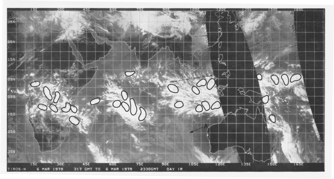
Figure 2. Sample Mercator projection mosaics of the IR-range satellite imagery (details as given in Fig. 1). All areas with highly reflective cloud cover, subjectively identified, are outlined.

There was a gap in the NOAA polar-orbiting satellite record between March 1978 and January 1979. That gap was filled by using satellite image mosaics from the Defense Meteorological Satellite Program (DMSP) archived at the World Data Center-A for Glaciology (Snow and Ice) in Boulder, Colorado. Those mosaics are Mercator projections at a scale of 1:15,000,000, covering 90° of latitude from 45° N to 45° S and averaging 52° of longitude. Twenty-one DMSP mosaics (seven each of visible, day IR, and night IR) are available for each 24-hour period. The larger scale for DMSP mosaics, compared with that for NOAA satellite mosaics (approximately 1:55,000,000), gives better resolution of cloud features.

Table 1. Satellites that produced the Mercator projection mosaics used as the basic source in deriving the HRC data set

                              Equator          Period          Number     
Satellite                     crossing         of record       of months  
                            (local time)                                  
--------------------------------------------------------------------------
ITOS-1, ESSA-9, NOAA-1       0900, 2100       1/71 - 5/74        41       

NOAA-SR series               0900, 2100       6/74 - 2/78        45       
  (NOAA-2, -3, -4, -5)                                                    

DMSP series                  Variable         3/78 - 1/79        11       

TIROS-N                      0330, 1530       2/79 - 1/80        12       

NOAA-6                       0730, 1930       2/80 - 8/81        19       

NOAA-7                       0230, 1430       9/81 - 1/85        41       

NOAA-9                       0230, 1430       2/85 - 12/85       11       
--------------------------------------------------------------------------
                                                                 180 Total

---

Analysis Procedures

The HRC data were analyzed to identify subjectively the location and extent of areas of organized convection by using daytime images from the polar-orbiting satellites. Whenever available, both visible and IR mosaics were used. Figure 3 depicts some of the common cloud types that can be observed in the mosaics and that are identified in Figures 1 and 2.

• Type A: Low-level stratus clouds that can appear bright in the visible-range mosaics, but are easily identified as nonconvective because they are gray in the IR mosaics (indicating a warm cloud top). They are large, persistent, and usually located near the west coast of a continent adjacent to a region of oceanic upwelling.

• Types D and E: Middle- to upper-level clouds generally associated with middle-latitude baroclinic zones and jetstreams that can frequently extend into the tropics, especially in the winter-season hemisphere. Type D clouds are thick cirrostratus; they appear bright in both the visible and IR mosaics, but they can be distinguished from HRC by their size, shape, texture, and location. Type E clouds are thin cirrostratus; they usually appear bright in the IR but gray in the visible.

• Types B and C: Cumulonimbus, true convective clouds that tend to produce copious rainfall when located in moist tropical environments. Both cloud types tend to have rather well-defined boundaries and appear bright in the visible and in the IR mosaics. Convective areas smaller than 200 km (type B) are considered too small to be coded as HRC for inclusion in the Atlas. True HRCs (type C) are highly reflective organized convective systems Of cumulonimbus clouds having a common cirrostratus shield extending more than 200 km horizontally; these HRCs are the subject of the Atlas.

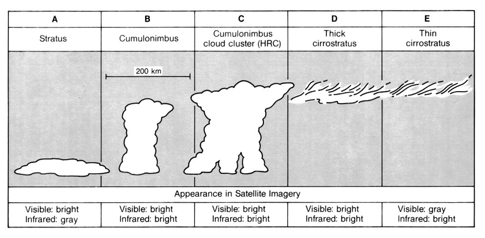
Figure 3. Cloud types illustrated in Figures 1 and 2, shown as vertical cross sections.

During the analysis procedure, a trained observer projects a microfilm image of a visible or an IR mosaic on a sheet of paper and outlines HRC areas (Fig. 2). The analyst takes into account factors such as the cloud size, appearance, and texture, variable background brightness, and local climatology, and applies overall knowledge of satellite meteorology. In general, an observer's experience constitutes a set of skills that is still virtually impossible to reproduce with computer algorithms, although developments in the field of expert systems may eventually change this.

After the HRC areas are analyzed for one day, the resulting data are digitized. The output of the digitizing procedure is a 51 x 360 array of grid squares of 1° latitude by 1° longitude, centered at the whole-degree intersections and extending from 25.5° N to 25.5° S around the globe. Grid squares covered by HRC are coded as 1 and all others as 0. No provision is made for different degrees of intensity of convective areas; each grid square is either covered by HRC (=1) or not covered (=0). After the daily data are digitized, the information is compressed into a packed binary format and stored in a cumulative computer file containing all the HRC data since January 1971.

There are frequent data gaps in the mosaic records (e.g., see Fig. 1). These gaps must be taken into account in any description of the frequency of occurrence of HRCs; consequently, areas without data were digitally recorded in a companion computer file.

---

Cautionary Notes

Effects of the 24-hour cycle of convection

The data presented in this Atlas reveal a tendency toward fewer days with HRC over land areas. This is especially noticeable in the difference between HRC over the large islands of Australasia and over the surrounding ocean areas. Presumably, these differences are mostly due to the 24-hour cycle of convection over land, where peak convective activity probably occurs during evening hours.

Consequences of subjective interpretation of data

Since the beginning of the project, different interpreters have subjectively analyzed HRC areas on the picture mosaics. In an effort to produce uniformity of analysis criteria, substantial portions of the data set were reanalyzed for this Atlas. Unfortunately, it is impossible to eliminate all subtle biases of a subjective analysis procedure. These biases, when accumulated over a month, can become significant. Systematic biases introduced by different analysts might also contribute to an increase in the monthly fields of coefficients of variation shown in Part II.

The average density of HRC

The maps of HRC presented in Part III show that the average amount of HRC present over the entire tropical belt varies considerably on a month-to-month basis. In fact, the general range of HRC coverage is 3% to 6%. Several factors may be responsible for this apparent variability, including the various satellite passage times over the years, regional differences in the 24-hour cycle of convection, systematic biases in the analysis of data, and possibly actual variability in the total amount of convection over the tropics. In view of this, changes in the patterns of HRC values from month to month should be considered more meaningful than changes in the average density.

The "edge" effect

The Mercator projection satellite picture mosaics from which the HRC data were derived are composed of two sections, each containing a hemisphere bounded by the dateline and the Greenwich meridian. HRC areas that straddle these two meridians are often broken into two sections in the analysis and digitizing procedures. As a result, there is a tendency to undercount HRC values in the grid squares immediately adjacent to these two meridians. This effect is especially noticeable in Parts I and II, and is purely an artifact of the processing of the data.

---

References

Conlan, E. F., 1973. Operational products from ITOS scanning radiometer data. NOAA Tech. Memo. NESS-52, NOAA National Environmental Satellite Service, Washington, D.C., 57 pp.

Garcia, 0., 1981. A comparison of two satellite rainfall estimates for GATE. J. Appl. Meteorol. 20:430-438.

Griffith, C. G., W. L. Woodley, J. S. Griffin, and S. C. Stromatt, 1980. Satellite-Derived Precipitation Atlas for GATE. NOAA Environmental Research Laboratories, Boulder, Colo., 280 pp.

Gruber, A., and A. F. Krueger, 1984. The status of the NOAA outgoing longwave radiation data set. Bull. Am. Meteorol. Soc. 65:958-962.

Houze, R. A., Jr., 1982. Cloud clusters and large-scale vertical motion in the tropics. J. Meteorol. Soc. Japan 60:396-410.

Janowiak, J. E., A. F. Krueger, P. A. Arkin, and A. Gruber, 1985. Atlas of Outgoing Longwave Radiation Derived from NOAA Satellite Data. NOAA Atlas No. 6, NOAA National Environmental Satellite, Data, and Information Service, Silver Spring, Md., 44 pp.

Kilonsky, B. J., and C. S. Ramage, 1976. A technique for estimating tropical open-ocean rainfall from satellite observations. J. Appl. Meteorol. 15:912-975.

Rasmusson, E. M., and J. M. Wallace, 1983. Meteorological aspects of the El Niño/Southern Oscillation. Science 222:1195-1202.