
The NOAA GML Carbon Cycle Group constructs Greenhouse Gas (GHG) Marine Boundary Layer (MBL) References using measurements of weekly air samples from the Cooperative Global Air Sampling Network [Conway et al., 1994; Dlugokencky et al., 1994; Novelli et al., 1992; Trolier et al., 1996]. References can be computed for nearly all long-lived trace gas species and isotopes routinely measured by NOAA and the University of Colorado Stable Isotope Laboratory. We describe how an MBL reference is constructed using measurements of CO2. References for other trace gas species and isotopes are computed using similar techniques.
The CO2 MBL reference is based on measurements from a subset of sites from the NOAA Cooperative Global Air Sampling Network. Only sites where samples are predominantly of well-mixed marine boundary layer (MBL) air representative of a large volume of the atmosphere are considered. These "MBL" sites are typically at remote marine sea level locations with prevailing onshore winds. Measurements from sites at altitude (e.g., Mauna Loa, Hawaii) and from sites close to anthropogenic and strong natural sources and sinks (e.g., Park Falls, Wisconsin) are excluded. Click here to see a map of sites used to construct the CO2 MBL reference.
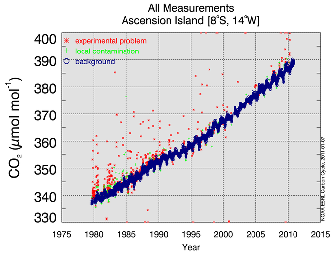
All measurements used to derive the CO2 reference are made by NOAA. Routine and ongoing comparison experiments within the Boulder lab help ensure that measurements are internally consistent with respect to calibration and methodology [WMO, 2009]. All data used to construct the MBL reference have been screened by the principal investigators. Only measurements determined to be free from sampling and analysis artifacts are used to construct the reference. Figure 1 shows all CO2 measurements of samples collected at Ascension Island.
To reduce noise in the determination of the MBL reference due to synoptic-scale atmospheric variability, we fit a smooth curve to the weekly measurements. To approximate the long-term trend and average seasonal cycle at a site (subscript “STA” for station), a function of the form
is fitted to the measurements [Thoning et al., 1989]. For CO2, the above function includes k=3 polynomial (quadratic) terms and nh=4 harmonic terms. The initial number of terms chosen can vary depending on the trace gas, the site and the sampling frequency. Click here to see the curve fitting parameters used to construct the CO2 MBL reference. To account for interannual variability in the seasonal cycle, the residuals, rSTA(t) = cSTA(t) - fSTA(t) where cSTA(t) denotes the actual observations, are digitally filtered through a low-pass filter with a full width at half maximum (FWHM) set to ~40 days. The smooth curve is then defined as
SSTA(t) = fSTA(t) + {rSTA(t)}40day
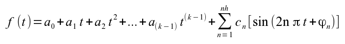
Figure 2 shows the smooth curve, S(t), fitted to background CO2 measurements from Ascension Island for 2000-2009. Click here to learn more about the Thoning et al. [1989] curve fitting methods.
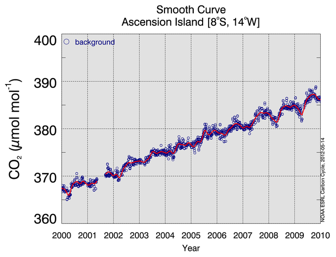
We use the data-based data extension methodology described by Masarie and Tans [1995] with important revisions documented in the GLOBALVIEW-CO2 [2011] to produce a set of extended records (one for each MBL dataset), which are synchronized in time and have no temporal gaps. For CO2, the synchronization period begins January 1, 1979 and ends when current year weekly air samples from the global network arrive at NOAA and can be measured. Extended records have 48 equal time steps per year; a time step is approximately 1 week (7.6 days). Figure 3 shows the Ascension Island extended record for 2000-2009.
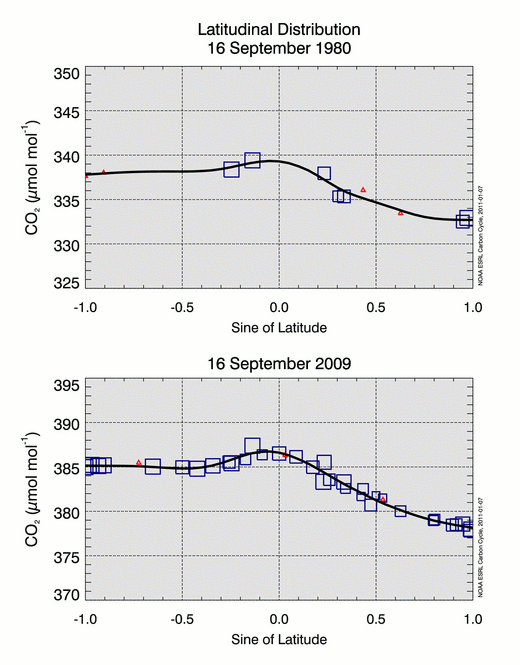
For each week in the synchronization period, we construct a latitude distribution (CO2 (ppm) versus sine of latitude) using smoothed and interpolated values from the set of MBL extended records. The number of values in the distribution can vary weekly as MBL sites are added to the NOAA network or terminated. Confidence in values extracted from the smooth curve, SSTA(t), depends on the density of the data, the “scatter” in the data and the length of the measurement period. We use a relative weighting scheme, which assigns greater significance to sites with high signal-to-noise and consistent sampling. Relative weights range from 1 to 10 where the minimum weight of 1 is reserved for all interpolated values. A curve is then fitted to each weekly weighted latitudinal distribution. Details of the latitudinal fitting process are described by Tans et al. [1989]. Figure 4 shows the fit to the latitudinal distributions for 16 September 1980 and 2009.
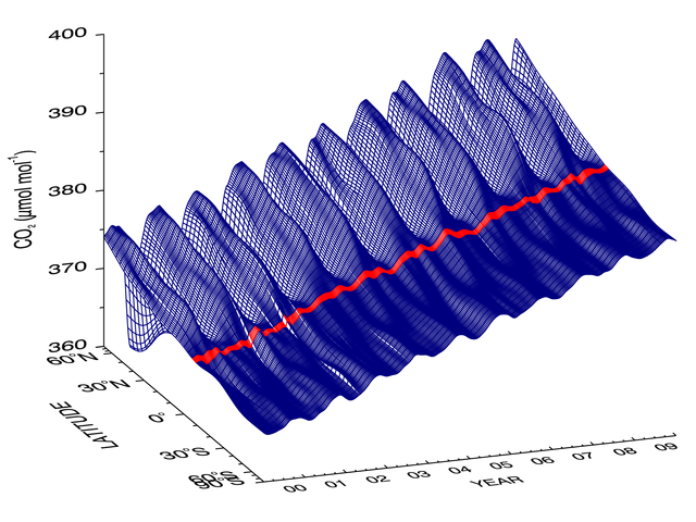
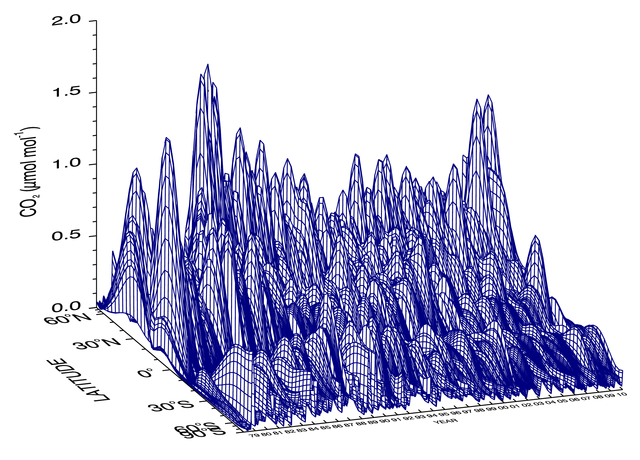
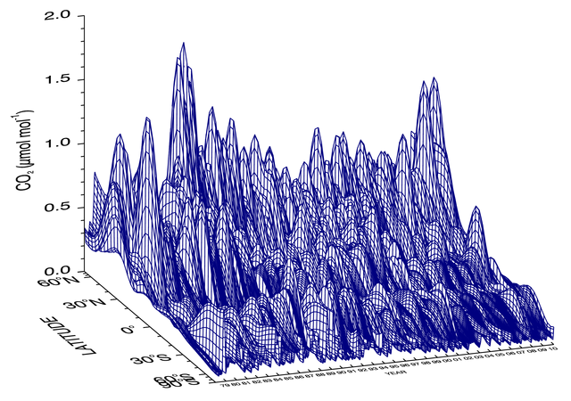
Values are extracted from each weekly latitudinal fit at intervals of 0.05 sine of latitude from 90ºS to 90ºN and joined together to create a 2-dimensional matrix (time versus latitude) of CO2 values. Figure 5 shows a three-dimensional representation of the global distribution of atmospheric CO2 derived using this methodology.
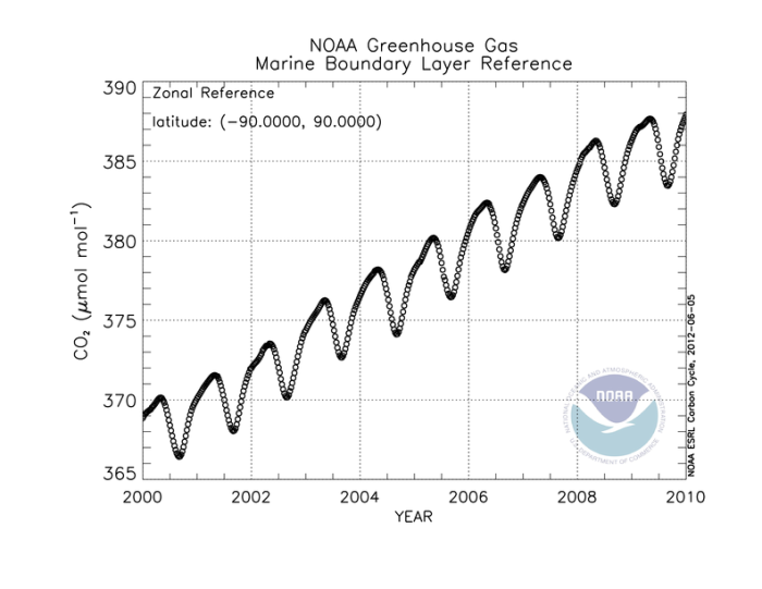
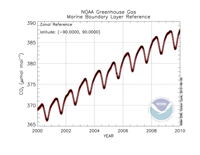
Using the above 2-dimensional reference matrix, we can construct a zonal-averaged time series for any specified latitude band or extract a time series at any specific latitude. The global mean CO2 MBL reference time series (Figure 6), for example, is created by computing, for each week, the latitude-weighted mean value for the band 90ºS to 90ºN.
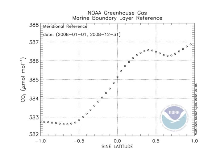
Using the 2-dimensional reference matrix, we can also construct a time-averaged meridional distribution over any latitude range. Figure 7 shows the 2008 annual average meridional distribution from 90°S to 90°N.
The MBL reference has uncertainty due to 1) lack of global coverage in the spatial distribution of MBL sites; 2) variability in atmospheric CO2 not adequately captured by weekly sampling; and 3) uncertainty in the actual measurements. Here we estimate the contribution from each of these sources of uncertainty.
The NOAA MBL reference is constructed from measurements of ~weekly samples collected at a subset of sites from the NOAA network. While the NOAA network is of global extent, it is currently too sparse to construct a reference that includes a longitudinal component using the described data-based methodology. Thus, we construct a reference that averages in latitude any observed variability in longitude (see Figure 4). Both the sparse network and the methodology may introduce bias in the reference. We estimate uncertainty in the reference due to the distribution of MBL sites using a bootstrap analysis [Conway et al., 1994].
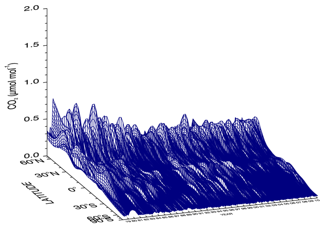
The CO2 reference is constructed using data from 42 MBL sites. We construct 100 bootstrap “networks” by choosing 42 sites randomly and with restitution from our set of MBL sites. In each network realization, some sites will be missing and some will be present two or more times. To ensure the meridional curve fits are adequately constrained by data, we require each bootstrap network to include (when available) at least one long-term record in each semi-hemisphere and in the Pacific and Atlantic Ocean basins. This constraint may differ for different compounds. We then apply the data extension methodology as described above to each of the 100 network realizations. Using the 100 reference matrices, we compute the mean and standard deviation at each time step and 0.05 sine of latitude. The standard deviation is our estimate of the uncertainty in the actual CO2 MBL reference. Figure 8 shows the 3-dimensional representation of the uncertainty estimate in the CO2 reference due to the MBL site distribution. This approach assumes the 100 network realizations are independent from one another, which is not the case. Our current estimate may increase slightly when we consider the correlation among the network realizations. A more comprehensive evaluation is currently underway.
The smooth curve, S(t), fitted to each MBL record reduces noise in the determination of the MBL reference by filtering out synoptic-scale atmospheric variability (see Section 2). Figure 9 shows atmospheric CO2 variability at Ascension Island not captured by S(t) from Figure 2. The residual distribution (S(t) minus data) includes variability related to synoptic scale weather patterns. We estimate uncertainty in the MBL reference due to atmospheric variability at each MBL site using a Monte Carlo analysis.
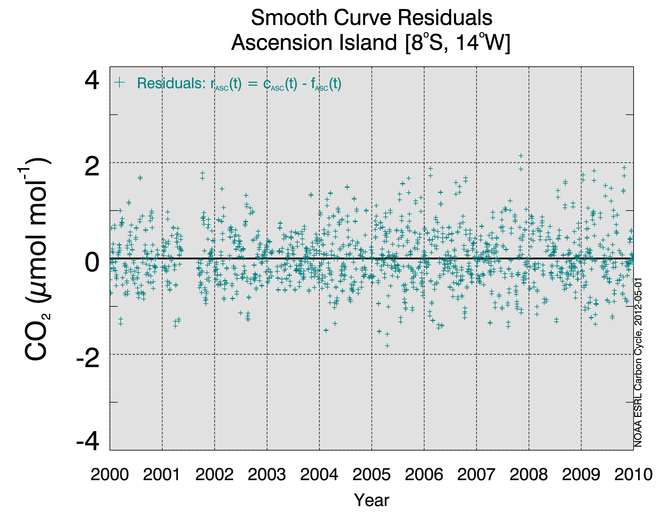
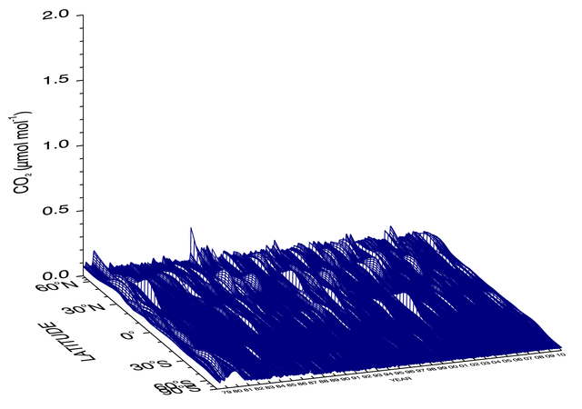
For each MBL record, we aggregate the residuals by month to compute an average monthly residual standard deviation (RSD). We then construct a new realization of the MBL record by adding a random error to the smooth curve value at each measurement time step. The random error is selected from a normal distribution with standard deviation equal to 1 and scaled by the average monthly RSD. For CO2, the lag 1 autocorrelation of the residuals was not statistically significant. A smooth curve fitted to this new record will differ from the original curve but will give the same residual statistics. We construct a reference using new realizations for each of the 42 MBL sites. We repeat this process 100 times. As before, we compute the mean and standard deviation at each time step and sine of latitude using the 100 reference matrices. Again, we use the standard deviation as our estimate of the uncertainty in the actual CO2 reference due to atmospheric variability. Figure 10 shows the 3-dimensional representation of the uncertainty estimate in the CO2 reference due to atmospheric variability at each MBL site.
The magnitude of reported measurement uncertainty for most greenhouse gas measurements made by NOAA and INSTAAR is typically much smaller than the atmospheric signals of interest. In general, measurement uncertainty has tended to decrease in time as instrumentation and methodology improve. We estimate uncertainty in the MBL reference due to measurement uncertainty using a Monte Carlo analysis.
Uncertainty in measurements of CO2 in weekly samples from the Cooperative Global Air Sampling Network has improved from ~0.2 ppm for measurements made prior to 1981, to 0.15 ppm from 1981 through 1987 to 0.10 ppm since. These estimates are based on measurements of “control” flasks filled from a well-calibrated high-pressure air cylinder and measured daily on the flask analytical system. Uncertainty in the propagation of the NOAA CO2 calibration scale is also included in these estimates and is small relative to the measurement reproducibility. Using these estimates, we construct a new realization of each MBL record by adding a random error to the smooth curve value at each measurement time step. The random error is selected from a normal distribution with standard deviation equal to 1 and scaled by the measurement uncertainty appropriate for the time step. A smooth curve fitted to this new record will differ from the original curve but will give residual statistics consistent with the estimated uncertainties. We construct a reference using new realizations for each of the 42 MBL sites. We repeat this process 100 times. As before, we compute the mean and standard deviation at each time step and sine of latitude using the 100 references. The standard deviation is our estimate of the uncertainty in the actual CO2 reference due to measurement uncertainty. Figure 11 shows the 3-dimensional representation of the uncertainty estimate in the CO2 MBL reference due to surface network measurement uncertainty.
We have estimated the uncertainty in the CO2 MBL reference due to 1) the spatial distribution of MBL sites; 2) variability in atmospheric CO2 not adequately captured by weekly sampling; and 3) uncertainty in the actual measurements. We can determine the effective uncertainty from the 3 sources combined. However, our uncertainty estimates due to atmospheric variability and measurement uncertainty are not independent. In fact, our estimate of uncertainty due to atmospheric variability includes uncertainty in our measurements. From Figures 10 and 11 we see that variability in atmospheric CO2 has a larger impact on the reference than measurement uncertainty. Again, this result may differ for different gases. We could difference the two 3-dimensional uncertainty distributions to separate atmospheric variability from measurement uncertainty, but this is not necessary for computing an overall uncertainty in the CO2 MBL reference. Instead, we assume uncertainties due to network distribution and our combined atmospheric variability and measurement uncertainty are independent, and compute an effective uncertainty by adding the 2 uncertainties in quadrature.
Figure 12 shows the 3-dimensional representation of the effective uncertainty in the CO2 MBL reference. Uncertainty due to our MBL network distribution dominates the combined uncertainty due to our measurements and atmospheric variability. This is an expected result and will likely decrease with a much denser network.
We use the effective uncertainty matrix to provide uncertainty estimates for products derived directly from the MBL reference. For example, Figure 13 shows the global mean CO2 MBL reference time series including uncertainty.
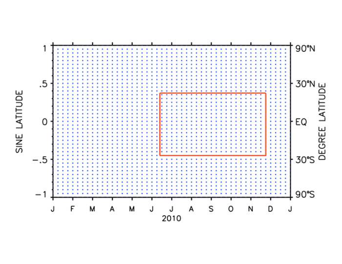
Products from this site are distributed as text files and include the requested reference, our best estimate of uncertainty, a citation reference, and PI contact information for follow up. Users may access the 3-dimensional MBL reference matrix and pre-defined or custom latitude-averaged time series and time-averaged meridional distributions. Custom references are constructed by specifying a date and/or latitude range (Figure 14). When the bounding region falls between the weekly and 0.05 sine of latitude steps of the matrix, intermediate values are determined using linear interpolation between bracketing values from the matrix. We use Simpson's Rule derived from the midpoint rectangle rule to compute the numerical integration for both zonal and meridional MBL references.
Please note: CO2, CH4, N2O and SF6 MBL references are available at this time.
The World Data Center for Greenhouse Gases also publishes global averages for CO2 and other gases. WDCGG uses curve fitting and data extension methods very similar to those developed by NOAA, but in addition to marine boundary layer sites, WDCGG includes many continental locations strongly influenced by local biospheric sources and sinks and also by fossil fuel emissions [Tsutsumi et al., 2009]. WDCGG also includes sites from multiple independent laboratories which raises the issue of possible artifacts due to differences in scale, sampling, gas handling, and detection techniques. The WDCCG global average has a positive mean offset of ~0.35 ppm and a larger seasonal cycle amplitude compared to NOAA results. The MBL estimate is expected to be lower than a full global surface average because areas with high fossil fuel loading due to recent emissions are not represented. On the other hand, the full troposphere (up to ~8-15 km altitude) and especially the stratosphere with lower CO2 mole fraction are not represented in either approach. We observe that CO2 is increasing at about the same rate everywhere it is measured. Because CO2 is a long lived gas in the atmosphere, any emission anywhere will in about one year’s time contribute to higher CO2 everywhere. One cannot “hide” CO2 emissions from the MBL sites for more than about a month. Thus the MBL reference gives probably the best low-noise representation of the ongoing global increase of CO2. We continue to base our global average on MBL sites because it is not clear how to properly weight continental sites in a global average. Our evidence so far indicates that the NOAA MBL global average is representative, internally consistent, and stable over time with respect to the addition of new MBL sites.