

CarbonTracker CT2013B
CarbonTracker is a CO2 measurement and modeling system developed by NOAA to keep track of sources (emissions to the atmosphere) and sinks (removal from the atmosphere) of carbon dioxide around the world. CarbonTracker uses atmospheric CO2 observations from a host of collaborators and simulated atmospheric transport to estimate these surface fluxes of CO2. The current release of CarbonTracker, CT2013B, provides global estimates of surface-atmosphere fluxes of CO2 from January 2000 through December 2012.
Executive Summary
Estimates of CO2 sources and sinks over North America
From 2001 through 2012, ecosystems in North America have been a net sink of 0.4 ± 1.3 PgC yr-1 (1 Petagram Carbon equals 1015 gC, or 1 billion metric ton C, or 3.67 billion metric ton CO2). This natural sink offsets about 20% of the emissions of about 1.8 PgC yr-1 from the burning of fossil fuels in the U.S.A., Canada and Mexico combined (Figure 1).

Whereas fossil emissions are generally steady over this period, ranging between 1.7 and 1.9 PgC yr-1, the amount of CO2 taken up by the North American biosphere varies significantly from year to year. In terrestrial biosphere models, inter-annual variability in land uptake can be related to anomalies in large-scale temperature and precipitation patterns. While the CarbonTracker period of analysis is relatively short compared to the dynamics of slowly-changing pools of biospheric carbon, episodes of extremes in net ecosystem exchange (NEE) have been associated with climatic anomalies (see e.g. Peters et al., 2007). It is interesting to note that the inferred year-to-year variabilty (the "range") of land uptake is actually as big as the mean sink itself.
Widespread droughts in the U.S. west and Canada during 2002 and 2012 resulted in relatively small annual uptake by terrestrial ecosystems in North America. In these years, land ecosystems were approximately neutral, neither emitting nor absorbing significant amounts of CO2. This should be compared with in an "average" year, in which these same land ecosystems remove about 0.4 PgC yr-1. The reduced land sinks in 2002 and 2012 are largely responsible for those years being the periods in the CarbonTracker record with the largest annual input of CO2 to the atmosphere from North America, when net emissions reached 1.8 ± 1.1 PgC yr-1.
The temperate North American region, basically comprising the United States, has been enduring a prolonged period of drought, and 2011 and 2012 were years where terrestrial ecosystems may have released carbon dioxide to the atmosphere. While fossil fuel emissions from the U.S. have not risen again to 2008 levels, 2011 and 2012 are the years with the largest net input of CO2 to the atmosphere.
Our observing system did not detect an effect from another significant drought, that in 2007 in the U.S. Southeast. This is likely due to lack of coverage of the area (Figure 3) in our current observing network. New observations in CT2013B compared to CT2009, however, do lead to interesting differences in this region for 2008. For CT2013B in 2008, the U.S. Southeast represents a distinct source of carbon dioxide to the atmosphere, whereas CT2009 fluxes for this same place and time are equivocal.
In CT2013B, we find that 2003 and 2004 were the years with the largest North American land sink, with ecosystems taking up about 0.6 PgC yr-1—a land sink that is about 70% bigger than the average. Fossil fuel emissions from North America were also slightly reduced in 2009 compared to earlier years as a result of the economic downturn. As a result, ecosystems removed about 28% of fossil fuel emissions over North America in 2009, and along with the highly-prductive 2003, this was the year with the lowest net input of CO2 to the atmosphere from North America. This 2009 net annual emission was 1.3 ± 1.0 PgC yr-1, about 15% smaller than the average of 1.5 ± 1.1 PgC yr-1.
Spatial distribution of surface fluxes
CarbonTracker flux estimates include sub-continental patterns of sources and sinks coupled to the distribution of dominant ecosystem types across the continent (Figure 2). We have greater confidence in countrywide totals than in estimates of regional sources and sinks, but we expect that such finer-scale estimates will become more robust with future expansion of the CO2 observing nework. Our results indicate that the sinks are mainly located in the agricultural regions of the U.S. and Canadian Midwest, and boreal forestsin Canada.

Word of caution about high-resolution biological flux maps
Figure 2 shows estimated fluxes by ecoregion. While we also provide flux maps and data with a finer 1° x 1° spatial resolution, for example on our flux maps pages, these ecoregions define the actual scales at which CarbonTracker operates. With the present observing network, the detailed one-degree fluxes should not be interpreted as quantitatively meaningful for each block. Any within-ecoregion patterns come directly from results of the terrestrial biosphere model. Part of this high-resolution patterning comes from variations of temperature, precipitation, light, plant species, and soil type over each ecoregion. To spread the influence of measurements from the sparse observation network, CarbonTracker makes adjustments uniformly over an entire ecoregion. These adjustments scale the net ecosystem flux of CO2 predicted by the terrestrial biosphere model by the same factor across each ecoregion. Thus we caution that the 1° x 1° spatial detail in CarbonTracker land fluxes is based on the simulations of the terrestrial biosphere model and the assumption of large-scale ecosystem coherence. This has not been verified by observations.
The CarbonTracker observing system
CarbonTracker surface flux estimates are optimally consistent with measurements of ~36,100 flask samples of air from 81 sites across the world, ~33,900 four-hourly averages of continuously measured CO2 at 13 sites (10 in North America, plus observatories at Mauna Loa, Hawaii; Barrow, Alaska, South Pole; and American Samoa), and ~15,100 four-hourly averages from towers at 9 locations within the continent (see Figure 3). Eight of these towers sample air from heights more than 100m above ground level.
Calculated time-dependent CO2 fields throughout the global atmosphere
A "byproduct" of the data assimilation system, once sources and sinks have been estimated, is that the mole fraction of CO2 is calculated everywhere in the model domain and over the entire 2000-2012 time period, based on the optimized source and sink estimates (Figure 4). As a check on model transport properties and CarbonTracker inversion performance, calculated CO2 mole fractions are regularly compared with measurements of ~31,000 air samples taken by NOAA/ESRL and collaborators at 30 aircraft sites, which are not used in the estimation of optimized sources and sinks.
Since CarbonTracker simulates CO2 throughout the entire atmospheric column, the model atmosphere can be sampled exactly like satellite retrievals of CO2. Such estimates are generally more sensitive to the CO2 mole fraction in some parts of the atmosphere than in others, and by using a vertical profile of this sensitivity, a direct analog of the satellite estimate can be constructed.
Flux uncertainties

It is important to note that at this time the uncertainty estimates for CarbonTracker sources and sinks are themselves quite uncertain. They have been derived from the mathematics of the ensemble data assimilation system, which requires several educated guesses for initial uncertainty estimates. The paper describing CarbonTracker (Peters et al. (2007), Proc. Nat. Acad. Sci. vol. 104, p. 18925-18930) presents different uncertainty estimates based on the sensitivity of the results to 14 alternative yet plausible ways to construct the CarbonTracker system. For example, the 14 realizations produce a range of the net annual mean terrestrial emissions in North America of -0.40 to -1.01 PgC -1 (negative emissions indicate a sink). The procedure is described in the Supporting Information Appendix to that paper, which is freely downloadable from the PNAS web site.
Furthermore, the estimates do not take into account several additional factors noted below. The calculation is set up for sources and sinks to slowly revert, in the absence of observational data, to first guesses of net ecosystem exchange, which are close to zero on an annual basis. This set-up may result in a bias. Also due to the sparseness of measurements, we have had to assume coherence of ecosystem processes over large distances, giving existing observations perhaps an undue amount of weight. The process model for terrestrial photosynthesis and respiration was very basic, and will likely be greatly improved in future releases of CarbonTracker. Easily the largest single annual mean source of CO2 is emissions from fossil fuel burning, which are currently not estimated by CarbonTracker. We use estimates from emissions inventories (economic accounting) and subtract the CO2 mole fraction signatures of those fluxes from observations. As a result, the biosphere and ocean fluxes estimated by CarbonTracker inherit error from the assumed fossil fuel emissions. While these emissions inventories may have a small relative error on global scales (perhaps 5 or 10%), any such bias translates into a larger relative error in the annual mean ecosystem sources and sinks, since those fluxes have smaller magnitudes. We expect to add a process model of fossil fuel combustion in future releases of CarbonTracker. Finally, additional measurement sites are expected to lead to the greatest improvements, especially to more robust and specific source/sink results at smaller spatial scales.
Consistency of modeled and observed atmospheric CO2 growth rates
Global atmospheric CO2 growth rates inferred directly from observed carbon dioxide at marine surface sites are consistent with those modeled by CarbonTracker, both in their average values and in their year-to-year variations (Figure 5). These global growth rates continue to hover at around 4 PgC yr-1, or around 1.9 ppm yr-1 (Figure 5). The 2009 growth rate modeled by CarbonTracker was below average at 3.4 ± 3.1 PgC yr-1. This was not due to a significant decrease in fossil fuel emissions, as can be seen from estimates of global fluxes used in CarbonTracker. Instead, the most notable difference for the 2009 atmospheric growth rate appears to be reduced biomass burning fluxes from the tropics and southern hemisphere, which at 1.4 PgC yr-1 are about 0.3 PgC yr-1 below their 2001-2012 mean of 1.7 PgC yr-1.

CT2013B methodological differences
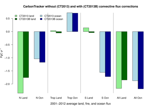
In each CarbonTracker simulation, fluxes are propagated to observation locations by a model of atmospheric transport. While it is known that there are errors and biases in this assumed transport, those issues are difficult to correct or to quantify. A significant improvement was made recently to the atmospheric transport model used in CarbonTracker. As a result of this "convective flux fix" (see relevant documentation), CT2013B surface flux estimates are significantly different than those of previous releases (see Figure 6). While global-scale fluxes remain basically unchanged, differences in regional fluxes are pronounced. These regional differences in long-term mean fluxes can be explored in our CarbonTracker version comparison tables. This is the most significant revision to CarbonTracker fluxes in the history of our program. It highlights the importance of accurate atmospheric transport in analysis of greenhouse gas concentrations, and comes as a direct result of comparing model simulations of other chemical species with observations (read more).
In CT2013B, CO2 uptake in temperate N. America (mainly U.S.) and Europe is reduced by about 0.6 PgC yr-1. This uptake is reapportioned about 50% to the worlds oceans and 50% to southern and tropical land regions. Notably, boreal uptake in N. America and Eurasia is not significantly impacted by this update.
CT2013B uses multiple "priors", or first-guess surface fluxes of CO2. In the CarbonTracker inversion system, first-guess fluxes are modified by comparison with observed atmospheric CO2 mole fractions. In any such Bayesian estimation system, the final flux result reflects, to some extent, influence of the prior. To evaluate the impact of the prior estimate on our final estimated fluxes, we have conducted eight independent simulations, each of which uses a unique combination of flux priors. This factorial design uses two different fossil fuel emissions estimates, two land biosphere models, and two air-sea exchange models.
We report here a statistical summary of that collection of simulations. Importantly, the reported uncertainty incorporates differences computed from this suite of eight independent simulations. Further information on the multi-model analysis is available in the CT2013B documentation:
This release of CarbonTracker is a full reanalysis of the 2000-2012 period.
2007 CarbonTracker PNAS publication
CarbonTracker is a NOAA contribution to the North American Carbon Program