Twenty Questions and Answers About the Ozone Layer: 2018 Update
Preface
The Twenty Questions and Answers About the Ozone Layer: 2018 Update is a component of the Scientific Assessment of Ozone Depletion: 2018 report. The report is prepared quadrennially by the Scientific Assessment Panel (SAP) of the Montreal Protocol on Substances that Deplete the Ozone Layer. The 2018 edition of the 20 Questions document is the fourth update of the original edition that appeared in the 2002 Assessment Report. The motivation behind this scientific publication is to tell the story of ozone depletion, ozone-depleting substances and the success of the Montreal Protocol. The questions and answers format divides the narrative into topics that can be read and studied individually by the intended audience of specialists and non-specialists. The topics range from the most basic (e.g., What is ozone?) to more recent developments (e.g., the Kigali Amendment). Each question begins with a short answer followed by a longer, more comprehensive answer. Figures enhance the narrative by illustrating key concepts and results. This document is principally based on scientific results presented in the 2018 and earlier Assessment Reports and has been extensively reviewed by scientists and non-specialists to ensure quality and readability.
We hope that you find this 20 Questions and Answers edition of value in communicating the scientific basis of ozone depletion and the success of the Montreal Protocol in protecting the ozone layer and future climate.
David W. Fahey, Paul A. Newman, John A. Pyle, and Bonfils Safari
Co-Chairs of the Scientific Assessment Panel
Lead Author
- Ross J. Salawitch, Department of Atmospheric and Oceanic Science & Department of Chemistry and Biochemistry, Earth System Science Interdisciplinary Center, University of Maryland, College Park, USA
- David W. Fahey, NOAA Earth System Research Laboratory, Chemical Sciences Division, USA
- Michaela I. Hegglin, University of Reading, UK
- Laura A. McBride, University of Maryland, College Park, USA
- Walter R. Tribett, University of Maryland, College Park, USA
- Sarah J. Doherty, University of Colorado, Cooperative Institute for Research in Environmental Sciences at NOAA Earth System Research Laboratory, Chemical Sciences Division, USA
Authors
See Appendix for Acknowledgements for the full list of contributors.
Introduction
Ozone is present only in small amounts in the atmosphere. Nevertheless, it is vital to human well-being as well as agricultural and ecosystem sustainability. Most of Earth's ozone resides in the stratosphere, the layer of the atmosphere that is more than 10 kilometers (6 miles) above the surface. About 90% of atmospheric ozone is contained in the stratospheric "ozone layer", which shields Earth's surface from harmful ultraviolet radiation emitted by the Sun.
In the mid-1970s scientists discovered that some human-produced chemicals could lead to depletion of the stratospheric ozone layer. The resulting increase in ultraviolet radiation at Earth's surface would increase the incidents of skin cancer and eye cataracts, and also adversely affect plants, crops, and ocean plankton.
Following the discovery of this environmental issue, researchers sought a better understanding of this threat to the ozone layer. Monitoring stations showed that the abundances of ozone-depleting substances (ODSs) were steadily increasing in the atmosphere. These trends were linked to growing production and use of chemicals like chlorofluorocarbons (CFCs) for spray can propellants, refrigeration and air conditioning, foam blowing, and industrial cleaning. Measurements in the laboratory and in the atmosphere characterized the chemical reactions that were involved in ozone destruction. Computer models of the atmosphere employing this information were used to simulate how much ozone depletion was already occurring and to predict how much more might occur in the future.
Observations of the ozone layer showed that depletion was indeed occurring. The most severe and most surprising ozone loss was discovered to be recurring in springtime over Antarctica. The loss in this region is commonly called the "ozone hole" because the ozone depletion is so large and localized. A thinning of the ozone layer also has been observed over other regions of the globe, such as the Arctic and northern and southern midlatitudes.
The work of many scientists throughout the world has built a broad and solid scientific understanding of the ozone depletion process. With this understanding, we know that ozone depletion is occurring and why. Most importantly, we know that if the most potent ODSs were to continue to be emitted and increase in the atmosphere, the result would be more depletion of the ozone layer.
In 1985 the world's governments adopted the Vienna Convention for the Protection of the Ozone Layer, in response to the prospect of increasing ozone depletion. The Vienna Convention provided a framework to protect the ozone layer. In 1987, this framework led to the Montreal Protocol on Substances that Deplete the Ozone Layer (the Montreal Protocol), an international treaty designed to control the production and consumption of CFCs and other ODSs. As a result of the broad compliance with the Montreal Protocol and its Amendments and Adjustments as well as industry's development of "ozone-friendly" substitutes to replace CFCs, the total global accumulation of ODSs in the atmosphere has slowed and begun to decrease. The replacement of CFCs has occurred in two phases: first via the use of hydrofluorocarbons (HCFCs) that cause considerably less damage to the ozone layer compared to CFCs, and second by the introduction of hydrofluorocarbons (HFCs) that pose no harm to ozone. In response, global ozone depletion has stabilized, and initial signs of recovery of the ozone layer have been identified. With continued compliance, substantial recovery of the ozone layer is expected by the middle of the 21st century. The day the Montreal Protocol was agreed upon, 16 September, is now celebrated as the International Day for the Preservation of the Ozone Layer.
The Amendment and Adjustment process is a vitally important aspect of the Montreal Protocol. At the Meeting of the Parties of the Montreal Protocol held in Kigali, Rwanda during October 2016, the Amendment process achieved an important new milestone, the Kigali Amendment. The Amendment phases down future global production and consumption of certain HFCs. While HFCs pose no threat to the ozone layer because they lack chlorine and bromine, they are greenhouse gases (GHGs), which lead to warming of surface climate. The amendment process was motivated by projections of substantial increases in the global use of HFCs in the coming decades. The control of HFCs under the Kigali Amendment marks the first time the Montreal Protocol has adopted regulations solely for the protection of climate.
The protection of the ozone layer and climate under the Montreal Protocol is a story of notable achievements: discovery, understanding, decisions, actions, and verification. It is a success story written by many: scientists, technologists, economists, legal experts, and policymakers, in which continuous dialogue has been a key ingredient. A timeline of milestones related to the science of stratospheric ozone depletion, international scientific assessments, and the Montreal Protocol is illustrated in Figure Q0-1.
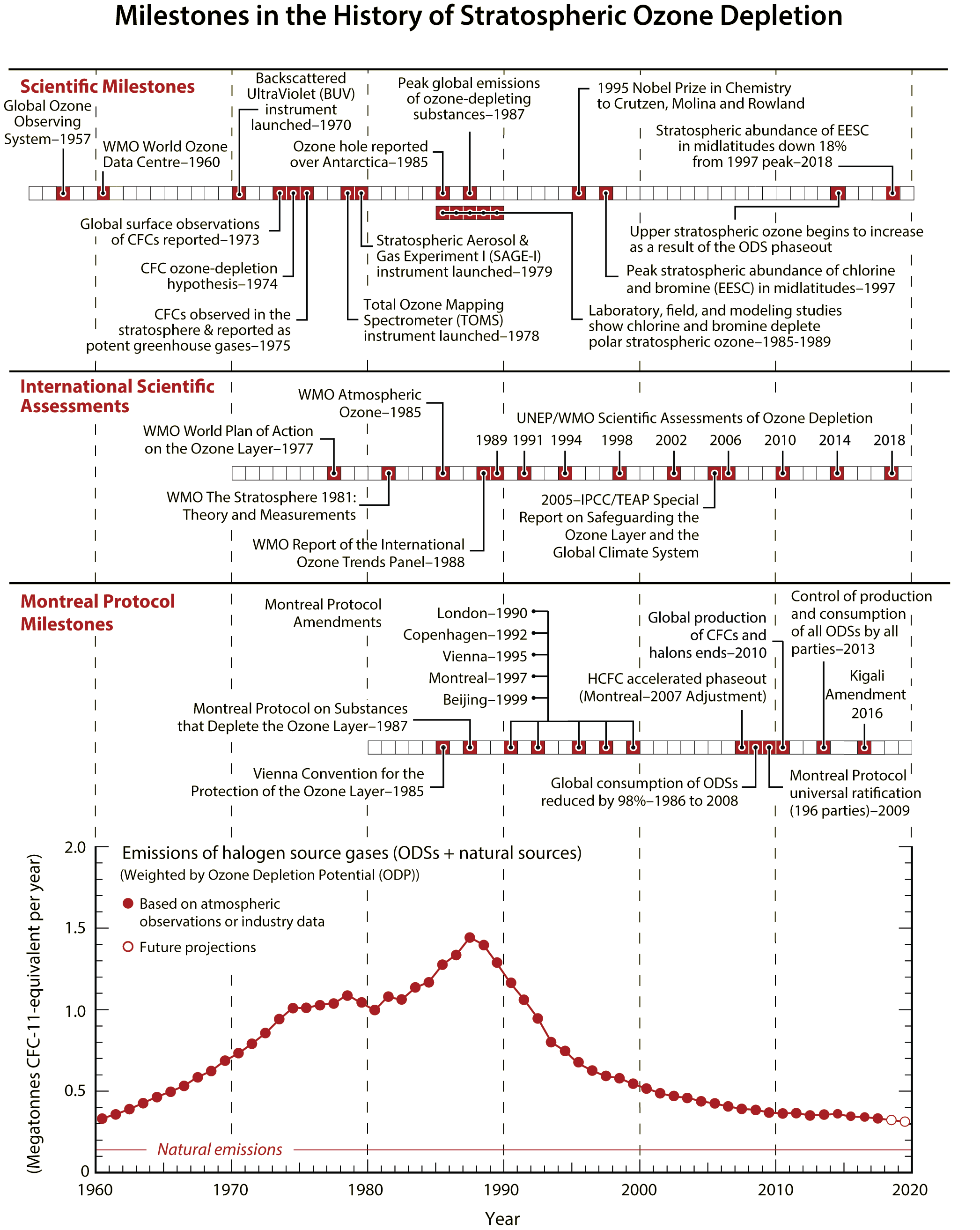
(A megatonne = 1 million (106) metric tons = 1 billion (109) kilograms.)
EESC: Equivalent effective stratospheric chlorine | IPCC: Intergovernmental Panel on Climate Change | ODS: Ozone-depleting substance | TEAP: Technology and Economic Assessment Panel of the Montreal Protocol | UNEP: United Nations Environment Programme |WMO: World Meteorological Organization
To help communicate the broad understanding of the Montreal Protocol, ODSs, and ozone depletion, as well as the relationship of these topics to GHGs and climate change, this component of the Scientfic Assessment of Ozone Depletion: 2018 describes the state of this science with 20 illustrated questions and answers. Most of the material is an update to that presented in previous Ozone Assessments. A new question has been added describing the expansion of climate protection under the Montreal Protocol (Q19).
The questions address the nature of atmospheric ozone, the chemicals that cause ozone depletion, how global and polar ozone depletion occur, the extent of ozone depletion, the success of the Montreal Protocol, the possible future of the ozone layer, and the protection against climate change that is now provided by the Kigali Amendment. Computer model projections show that GHGs and changes in climate will have a growing in uence on global ozone in the coming decades, and in some cases will exceed the in uence of ODSs in most atmospheric regions by the end of this century. Ozone and climate are indirectly linked because both ODSs and their substitutes as well as ozone itself are GHGs that contribute to climate change.
A brief answer to each question is first given in dark red; an expanded answer then follows. The answers are based on the information presented in the 2018 and earlier Assessment reports as well as other international scientfic assessments. These reports and the answers provided here were prepared and reviewed by a large number of international scientists who are experts in different research fields related to the science of stratospheric ozone and climate1.
1 See Appendix for Acknowledgments.
Ozone in our atmosphere
Ozone is a gas that is naturally present in our atmosphere. Each ozone molecule contains three atoms of oxygen and is denoted chemically as O3. Ozone is found primarily in two regions of the atmosphere. About 10% of Earth’s ozone is in the troposphere, which extends from the surface to about 10–15 kilometers (6–9 miles) altitude. About 90% of Earth’s ozone resides in the stratosphere, the region of the atmosphere between the top of the troposphere and about 50 kilometers (31 miles) altitude. The part of the stratosphere with the highest amount of ozone is commonly referred to as the “ozone layer”. Throughout the atmosphere, ozone is formed in multistep chemical processes that are initiated by sunlight. In the stratosphere, the process begins with an oxygen molecule (O2 ) being broken apart by ultraviolet radiation from the Sun. In the troposphere, ozone is formed by a different set of chemical reactions that involve naturally occurring gases as well as those from sources of air pollution.
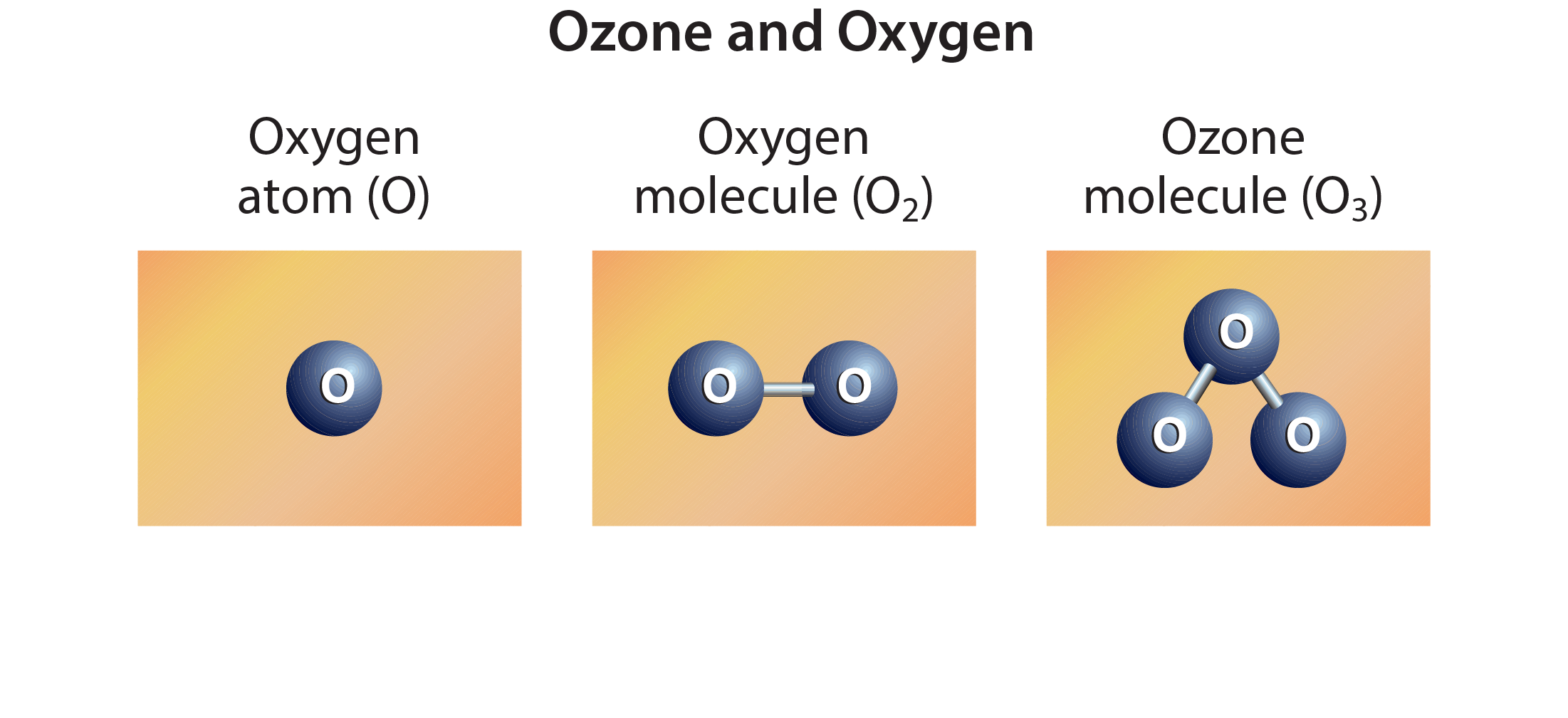
Ozone is a gas that is naturally present in our atmosphere. Ozone has the chemical formula O3 because an ozone molecule contains three oxygen atoms (see Figure Q1-1). Ozone was discovered in laboratory experiments in the mid-1800s. Ozone’s presence in the atmosphere was later discovered using chemical and optical measurement methods. The word ozone is derived from the Greek word óζειν (ozein), meaning “to smell.” Ozone has a pungent odor that allows it to be detected even at very low amounts. Ozone reacts rapidly with many chemical compounds and is explosive in concentrated amounts. Electrical discharges are generally used to produce ozone for industrial processes such as air and water purification and bleaching of textiles and food products.
Ozone location. Most ozone (about 90%) is found in the stratosphere, which begins about 10–15 kilometers (km) above Earth’s surface and extends up to about 50 km altitude. The stratospheric region with the highest concentration of ozone, between about 15 and 35 km altitude, is commonly known as the “ozone layer” (see Figure Q1-2). The ozone layer extends over the entire globe with some variation in altitude and thickness. Most of the remaining ozone (about 10%) is found in the troposphere, which is the lowest region of the atmosphere, between Earth’s surface and the stratosphere. Tropospheric air is the “air we breathe” and, as such, excess ozone in the troposphere has harmful consequences (see Q2).
Ozone abundance. Ozone molecules have a low relative abundance in the atmosphere. Most air molecules are either oxygen (O2) or nitrogen (N2). In the stratosphere near the peak concentration of the ozone layer, there are typically a few thousand ozone molecules for every billion air molecules (1 billion = 1,000 million). In the troposphere near Earth’s surface, ozone is even less abundant, with a typical range of 20 to 100 ozone molecules for each billion air molecules. The highest ozone values near the surface occur in air that is polluted by human activities.
As an illustration of the low relative abundance of ozone in our atmosphere, one can imagine bringing all the ozone molecules in the troposphere and stratosphere down to Earth’s surface and forming a layer of pure ozone that extends over the entire globe. The resulting layer would have an average thickness of about three millimeters (0.12 inches) (see Q3). Nonetheless, this extremely small fraction of the atmosphere plays a vital role in protecting life on Earth (see Q2).

Stratospheric ozone. Stratospheric ozone is formed naturally by chemical reactions involving solar ultraviolet radiation (sunlight) and oxygen molecules, which make up about 21% of the atmosphere. In the first step, solar ultraviolet radiation breaks apart one oxygen molecule (O2) to produce two oxygen atoms (2 O) (see Figure Q1-3). In the second step, each of these highly reactive oxygen atoms combines with an oxygen molecule to produce an ozone molecule (O3). These reactions occur continually whenever solar ultraviolet radiation is present in the stratosphere. As a result, the largest ozone production occurs in the tropical stratosphere.
The production of stratospheric ozone is balanced by its destruction in chemical reactions. Ozone reacts continually with sunlight and a wide variety of natural and human-produced chemicals in the stratosphere. In each reaction, an ozone molecule is lost and other chemical compounds are produced. Important reactive gases that destroy ozone are hydrogen and nitrogen oxides and those containing chlorine and bromine (see Q7). Some stratospheric ozone is regularly transported down into the troposphere and can occasionally influence ozone amounts at Earth’s surface.
Tropospheric ozone. Near Earth’s surface, ozone is produced by chemical reactions involving gases emitted to the atmosphere from both natural sources and human activities. Ozone production reactions primarily involve hydrocarbon and nitrogen oxide gases, as well as ozone itself, and all require sunlight for completion. Fossil fuel combustion is a primary source of pollutant gases that lead to tropospheric ozone production. As in the stratosphere, ozone in the troposphere is destroyed by naturally occurring chemical reactions and by reactions involving human-produced chemicals. Tropospheric ozone can also be destroyed when ozone reacts with a variety of surfaces, such as those of soils and plants.
Balance of chemical processes. Ozone abundances in the stratosphere and troposphere are determined by the balance between chemical processes that produce and destroy ozone. The balance is determined by the amounts of reactive gases and how the rate or effectiveness of the various reactions varies with sunlight intensity, location in the atmosphere, temperature, and other factors. As atmospheric conditions change to favor ozone-producing reactions in a certain location, ozone abundances increase. Similarly, if conditions change to favor other reactions that destroy ozone, abundances decrease. The balance of production and loss reactions, combined with atmospheric air motions that transport and mix air with different ozone abundances, determines the global distribution of ozone on timescales of days to many months (see also Q3). Global stratospheric ozone has decreased during the past several decades (see Q12) because the amounts of reactive gases containing chlorine and bromine have increased in the stratosphere due to human activities (see Q6 and Q15).

Ozone in the stratosphere absorbs a large part of the Sun’s biologically harmful ultraviolet radiation. Stratospheric ozone is considered “good” ozone because of this beneficial role. In contrast, ozone formed at Earth’s surface in excess of natural amounts is considered “bad” ozone because it is harmful to humans, plants, and animals.
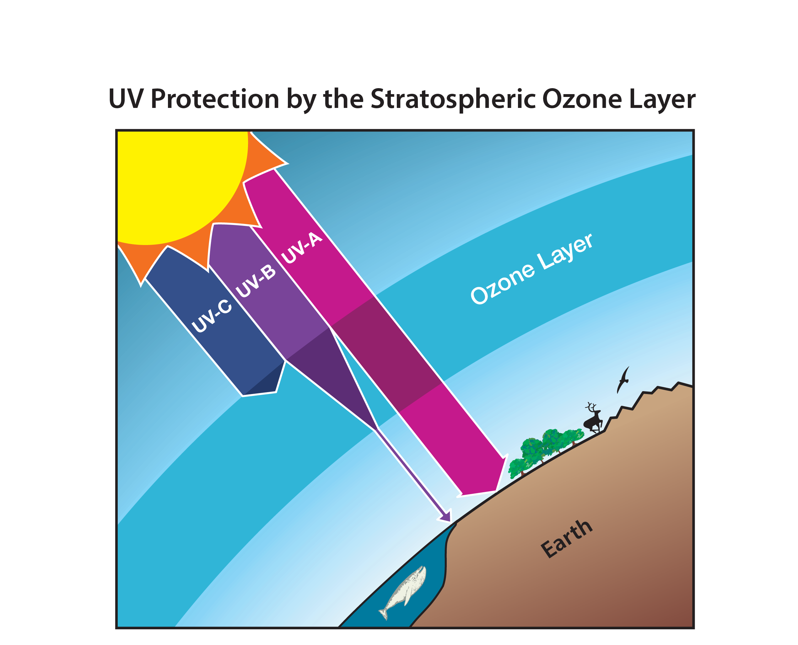
Ozone in the stratosphere (Good ozone). Stratospheric ozone is considered good for humans and other life forms because it absorbs ultraviolet (UV) radiation from the Sun (see Figure Q2-1). If not absorbed, high energy UV radiation would reach Earth’s surface in amounts that are harmful to a variety of life forms. The Sun emits three types of UV radiation: UV-C (100 to 280 nanometer (nm) wavelengths); UV-B (280 to 315 nm), and UV-A (315 to 400 nm). Exposure to UV-C radiation is particularly dangerous to all life forms. Fortunately, UV-C radiation is entirely absorbed within the ozone layer. Most UV-B radiation emitted by the Sun is absorbed by the ozone layer; the rest reaches Earth’s surface. In humans, increased exposure to UV-B radiation raises the risks of skin cancer and cataracts, and suppresses the immune system. Exposure to UV-B radiation before adulthood and cumulative exposure are both important health risk factors. Excessive UV-B exposure also can damage terrestrial plant life, including agricultural crops, single-celled organisms, and aquatic ecosystems. Low energy UV radiation, UV-A, which is not absorbed significantly by the ozone layer, causes premature aging of the skin.
Protecting stratospheric ozone. In the mid-1970s, it was discovered that gases containing chlorine and bromine atoms released by human activities could cause stratospheric ozone depletion (see Q5 and Q6). These gases, referred to as halogen source gases, and also as ozone-depleting substances (ODSs), chemically release their chlorine and bromine atoms after they reach the stratosphere. Ozone depletion increases surface UV-B radiation above naturally occurring amounts. International efforts have been successful in protecting the ozone layer through controls on the production and consumption of ODSs (see Q14 and Q15).
(The unit “nanometer” (nm) is a common measure of the wavelength of light; 1 nm equals one billionth of a meter (=10-9 m).)
Ozone in the troposphere (Bad ozone). Ozone near Earth’s surface in excess of natural amounts is considered bad ozone (see Figure Q1-2). Surface ozone in excess of natural levels is formed by reactions involving air pollutants emitted from human activities, such as nitrogen oxides (NOx), carbon monoxide (CO), and various hydrocarbons (gases containing hydrogen, carbon, and often oxygen). Exposure to surface ozone above natural levels is harmful to humans, plants, and other living systems because ozone reacts strongly to destroy or alter many biological molecules. Enhanced surface ozone caused by air pollution reduces crop yields and forest growth. In humans, exposure to high levels of ozone can reduce lung capacity; cause chest pains, throat irritation, and coughing; and worsen pre-existing health conditions related to the heart and lungs. In addition, increases in tropospheric ozone lead to a warming of Earth’s surface because ozone is a greenhouse gas (GHG) (see Q17). The negative effects of excess tropospheric ozone contrast sharply with the protection from harmful UV radiation afforded by preserving the natural abundance of stratospheric ozone.
Reducing tropospheric ozone. Limiting the emission of certain common pollutants reduces the production of excess ozone near Earth’s surface where it can affect humans, plants, and animals. Major sources of pollutants include large cities where fossil fuel consumption and industrial activities are greatest. Many programs around the globe have been successful in reducing or limiting the emission of pollutants that cause production of excess ozone near Earth’s surface.
Natural ozone. In the absence of human activities, ozone would still be present near Earth’s surface and throughout the troposphere and stratosphere because ozone is a natural component of the clean atmosphere. Natural emissions from the biosphere, mainly from trees, participate in chemical reactions that produce ozone. Atmospheric ozone plays important ecological roles beyond absorbing UV radiation. For example, ozone initiates the chemical removal of many pollutants as well as some GHGs, such as methane (CH4). In addition, the absorption of UV radiation by ozone is a natural source of heat in the stratosphere, causing temperatures to increase with altitude. Stratospheric temperatures affect the balance of ozone production and destruction processes (see Q1) and air motions that redistribute ozone throughout the stratosphere (see Q3).
The distribution of total ozone over Earth varies with geographic location and on daily to seasonal timescales. These variations are caused by large-scale movements of stratospheric air and the chemical production and destruction of ozone. Total ozone is generally lowest at the equator and highest in midlatitude and polar regions.
Total ozone. The total ozone column at any location on the globe is defined as the sum of all the ozone in the atmosphere directly above that location. Most ozone resides in the stratospheric ozone layer and a small percentage (about 10%) is distributed throughout the troposphere (see Q1). Total ozone column values are often reported in Dobson units denoted as “DU.” Typical values vary between 200 and 500 DU over the globe, with a global average abundance of about 300 DU (see Figure Q3-1). The quantity of ozone molecules required for total ozone to be 300 DU could form a layer of pure ozone gas at Earth’s surface having a thickness of only 3 millimeters (0.12 inches) (see Q1), which is about the height of a stack of 2 common coins. It is remarkable that a layer of pure ozone only 3 millimeters thick protects life on Earth’s surface from harmful UV radiation emitted by the Sun (see Q2).
Global distribution. Total ozone varies strongly with latitude over the globe, with the largest values occurring at middle and high latitudes during most of the year (see Figure Q3-1). This distribution is the result of the large-scale circulation of air in the stratosphere that slowly transports ozone from the tropics, where ozone production from solar ultraviolet radiation is highest, toward the poles. Ozone accumulates at middle and high latitudes, increasing the vertical extent of the ozone layer and, at the same time, total ozone. Values of total ozone are generally smallest in the tropics for all seasons. An exception in recent decades is the region of low values of ozone over Antarctica during spring in the Southern Hemisphere, a phenomenon known as the Antarctic ozone hole (dark blue, Figure Q3-1; also see Q10 and Q11).
Seasonal distribution. Total ozone also varies with season, as shown in Figure Q3-1 using two-week averages of ozone taken from 2009 satellite observations. March and September plots represent the early spring and autumn seasons in the Northern and Southern Hemispheres. June and December plots similarly represent the early summer and winter seasons. During spring, total ozone exhibits maximums at latitudes poleward of about 45° N in the Northern Hemisphere and between 45° and 60° S in the Southern Hemisphere. These spring maximums are a result of increased transport of ozone from its source region in the tropics toward high latitudes during late autumn and winter. This poleward ozone transport is much weaker during the summer and early autumn periods and is weaker overall in the Southern Hemisphere.
This natural seasonal cycle can be observed clearly in the Northern Hemisphere as shown in Figure Q3-1, with increasing values in Arctic total ozone during winter, a clear maximum in spring, and decreasing values from summer to autumn. In the Antarctic, however, a pronounced minimum in total ozone is observed during spring. The minimum is known as the “ozone hole”, which is caused by the widespread chemical depletion of ozone in spring by pollutants known as ozone-depleting substances (see Q5 and Q10). In the late 1970s, before the ozone hole appeared each year, much higher ozone values than those currently observed were found in the Antarctic spring (see Q10). Now, the lowest values of total ozone across the globe and all seasons are found every late winter/early spring in the Antarctic as shown in Figure Q3-1. After spring, these low values disappear from total ozone maps as polar air mixes with lower-latitude air containing much higher amounts of ozone.
In the tropics, the change in total ozone through the progression of the seasons is much smaller than in the polar regions. This feature is due to seasonal changes in both sunlight and ozone transport being much smaller in the tropics compared to polar regions.
Natural variations. Total ozone varies strongly with latitude and longitude as seen within the seasonal plots in Figure Q3-1. These patterns come about for two reasons. First, atmospheric winds transport air between regions of the stratosphere that have high ozone values and those that have low ozone values. Tropospheric weather systems can temporarily alter the vertical extent of the ozone layer in a region, and thereby change total ozone. The regular nature of these air motions, in some cases associated with geographical features (oceans and mountains), in turn causes recurring patterns in the distribution of total ozone.
Second, ozone variations occur as a result of changes in the balance of chemical production and loss processes as air moves to and from different locations over the globe. This balance, for example, is very sensitive to the amount of sunlight in a region.
There is a good understanding of how chemistry and air motions work together to cause the observed large-scale features in total ozone, such as those seen in Figure Q3-1. Ozone changes are routinely monitored by a large group of investigators using satellite, airborne, and ground-based instruments. The continued analyses of these observations provide an important basis to quantify the contribution of human activities to ozone depletion.

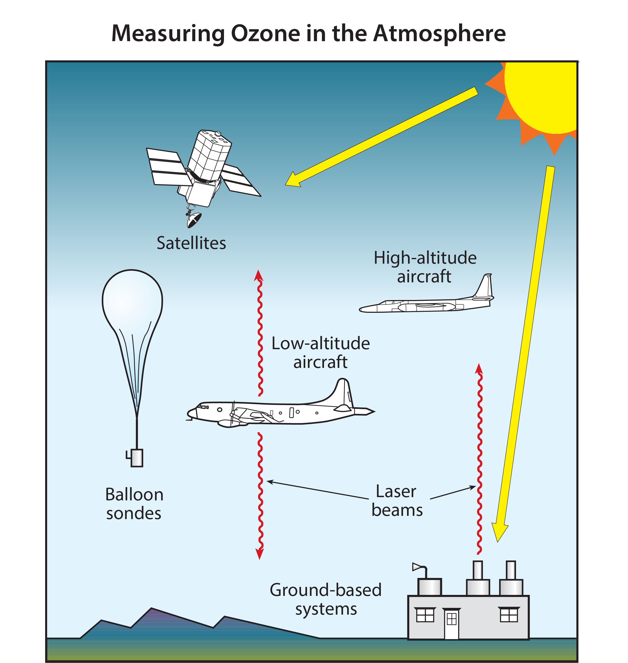
The amount of ozone in the atmosphere is measured by instruments on the ground and carried aloft on balloons, aircraft, and satellites. Some instruments measure ozone locally by continuously drawing air samples into a small detection chamber. Other instruments measure ozone remotely over long distances by using ozone’s unique optical absorption or emission properties.
The abundance of ozone in the atmosphere is measured by a variety of techniques (see Figure Q4-1). The techniques make use of ozone’s unique optical and chemical properties. There are two principal categories of measurement techniques: local and remote. Ozone measurements by these techniques have been essential in monitoring changes in the ozone layer and in developing our understanding of the processes that control ozone abundances.
Local measurements. Local measurements of the atmospheric abundance of ozone are those that require air to be drawn directly into an instrument. Once inside an instrument’s detection chamber, the amount of ozone is determined by measuring the absorption of ultraviolet (UV) light or by the electrical current or light produced in a chemical reaction involving ozone. The last approach is used in “ozonesondes” that are lightweight, ozone-measuring modules suitable for launching on small balloons. The balloons ascend up to altitudes of about 32 to 35 kilometers (km), high enough to measure ozone in the stratospheric ozone layer. Ozonesondes are launched regularly at many locations around the world. Local ozone-measuring instruments using optical or chemical detection schemes are also used on research aircraft to measure the distribution of ozone in the troposphere and lower stratosphere (up to altitudes of about 20 km). High-altitude research aircraft can reach the ozone layer at most locations over the globe and can reach furthest into the layer at high latitudes. Ozone measurements are also being made routinely on some commercial aircraft flights.
Remote measurements. Remote measurements of total ozone amounts and the altitude distributions of ozone are obtained by detecting ozone at large distances from the instrument. Most remote measurements of ozone rely on its unique absorption of UV radiation. Sources of UV radiation that can be used are the Sun, lasers, and starlight. For example, satellite instruments use the absorption of solar UV radiation by the atmosphere or the absorption of sunlight scattered from the surface of Earth to measure ozone over nearly the entire globe on a daily basis. Lidar instruments, which measure backscattered laser light, are routinely deployed at ground sites and on research aircraft to detect ozone over a distance of many kilometers along the laser light path. A network of ground-based detectors measures ozone by detecting small changes in the amount of the Sun’s UV radiation that reaches Earth’s surface. Other instruments measure ozone using its absorption of infrared or visible radiation or its emission of microwave or infrared radiation at different altitudes in the atmosphere, thereby obtaining information on the vertical distribution of ozone. Emission measurements have the advantage of providing remote ozone measurements at night, which is particularly valuable for sampling polar regions during winter, when there is continuous darkness.
The ozone depletion process
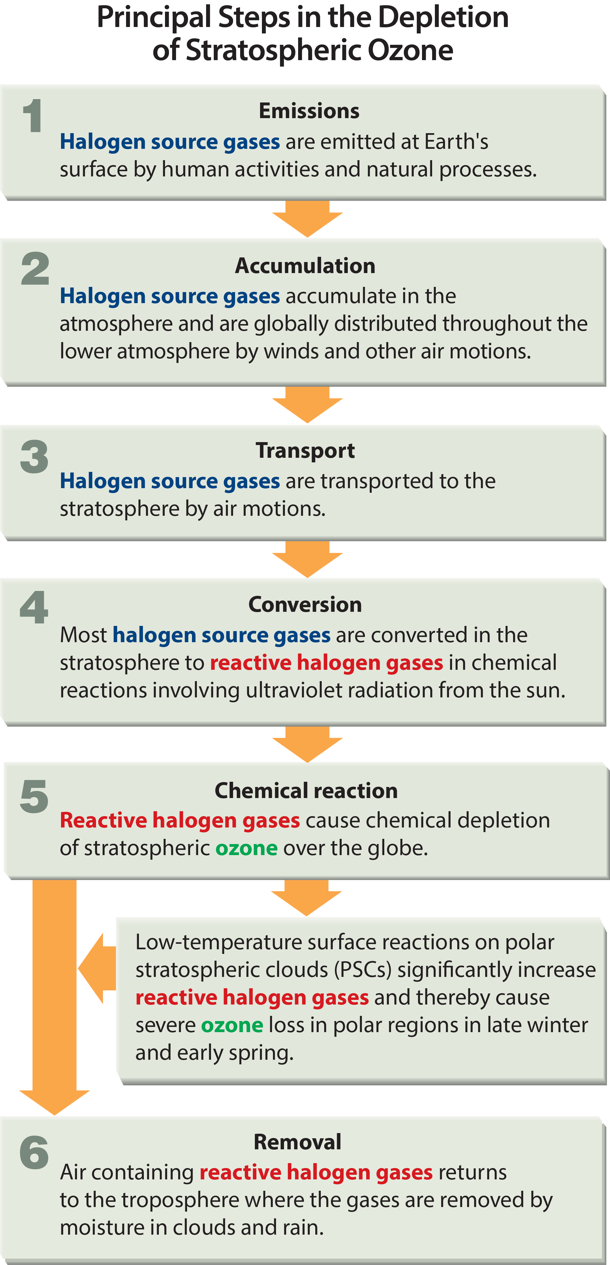
The initial step in the depletion of stratospheric ozone by human activities is the emission, at Earth’s surface, of gases that contain chlorine and bromine and have long atmospheric lifetimes. Most of these gases accumulate in the lower atmosphere because they are relatively unreactive and do not dissolve readily in rain or snow. Natural air motions transport these accumulated gases to the stratosphere, where they are converted to more reactive gases. Some of these gases then participate in reactions that destroy ozone. Finally, when air returns to the lower atmosphere, these reactive chlorine and bromine gases are removed from Earth’s atmosphere by rain and snow.
Emission, accumulation, and transport. The principal steps in stratospheric ozone depletion caused by human activities are shown in Figure Q5-1. The process begins with the emission, at Earth’s surface, of long-lived source gases containing the halogens chlorine and bromine (see Q6). The halogen source gases, often referred to as ozone-depleting substances (ODSs), include manufactured chemicals released to the atmosphere in a variety of applications, such as refrigeration, air conditioning, and foam blowing. Chlorofluorocarbons (CFCs) are an important example of a chlorine-containing source gas. Emitted source gases accumulate in the lower atmosphere (troposphere) and are transported to the stratosphere by natural air motions. The accumulation occurs because most source gases are highly unreactive in the lower atmosphere. Small amounts of these gases dissolve in ocean waters. The low reactivity of these manufactured halogenated gases is one property that made them well suited for specialized applications such as refrigeration.
Some halogen gases are emitted in substantial quantities from natural sources (see Q6). These emissions also accumulate in the troposphere, are transported to the stratosphere, and participate in ozone destruction reactions. These naturally emitted gases are part of the natural balance of ozone production and destruction that predates the large release of manufactured halogenated gases.
Conversion, reaction, and removal. Halogen source gases do not react directly with ozone. Once in the stratosphere, halogen source gases are chemically converted to reactive halogen gases by ultraviolet radiation from the Sun (see Q7). The rate of conversion is related to the atmospheric lifetime of a gas (see Q6). Gases with longer lifetimes have slower conversion rates and survive longer in the atmosphere after emission. Lifetimes of the principal ODSs vary from about 1 to 100 years (see Table Q6-1). Emitted gas molecules with atmospheric lifetimes greater than a few years circulate between the troposphere and stratosphere multiple times, on average, before conversion occurs.
The reactive gases formed from halogen source gases react chemically to destroy ozone in the stratosphere (see Q8). The average depletion of total ozone attributed to reactive gases is smallest in the tropics and largest at high latitudes (see Q12). In polar regions, surface reactions that occur at low temperatures on polar stratospheric clouds greatly increase the abundance of the most reactive chlorine gas, chlorine monoxide (ClO) (see Q9). This process results in substantial ozone destruction in polar regions in late winter/early spring (see Q10 and Q11).
After a few years, air in the stratosphere returns to the troposphere, bringing along reactive halogen gases. These reactive halogen gases are then removed from the atmosphere by rain and other precipitation or deposited on Earth’s land or ocean surfaces. This removal brings to an end the destruction of ozone by chlorine and bromine atoms that were first released to the atmosphere as components of halogen source gas molecules.
Tropospheric conversion. Halogen source gases with short lifetimes (less than 1 year) undergo significant chemical conversion in the troposphere, producing reactive halogen gases and other compounds. Source gas molecules that are not converted are transported to the stratosphere. Only small portions of reactive halogen gases produced in the troposphere are transported to the stratosphere because most are removed by precipitation. Important examples of halogen gases that undergo some tropospheric removal are the hydrochlorofluorocarbons (HCFCs), methyl bromide (CH3Br), methyl chloride (CH3Cl), and gases containing iodine (see Q6).
Certain industrial processes and consumer products result in the emission of ozone-depleting substances (ODSs) to the atmosphere. ODSs are manufactured halogen source gases that are controlled worldwide by the Montreal Protocol. These gases bring chlorine and bromine atoms to the stratosphere, where they destroy ozone in chemical reactions. Important examples are the chlorofluorocarbons (CFCs), once used in almost all refrigeration and air conditioning systems, and the halons, which were used as fire extinguishing agents. Current ODS abundances in the atmosphere are known directly from air sample measurements.
Halogen source gases versus ozone-depleting substances (ODSs). Those halogen source gases emitted by human activities and controlled by the Montreal Protocol are referred to as ODSs within the Montreal Protocol, by the media, and in the scientific literature. The Montreal Protocol controls the global production and consumption of ODSs (see Q14). Halogen source gases such as methyl chloride (CH3Cl) that have predominantly natural sources are not classified as ODSs. The contributions of ODSs and natural halogen source gases to the total amount of chlorine and bromine entering the stratosphere, which peaked in 1993 and 1998, respectively, are shown in Figure Q6-1. The difference in the timing of the peaks is a result of different phaseout schedules specified by the Montreal Protocol, atmospheric lifetimes, and the time delays between production and emissions of the various source gases. Also shown are the contributions to total chlorine and bromine in 2016, highlighting the reductions of 10% and 11%, respectively, achieved under the controls of the Montreal Protocol.
Ozone-depleting substances (ODSs). ODSs are manufactured for specific industrial uses or consumer products, most of which result in the eventual emission of these gases to the atmosphere. Total ODS emissions increased substantially from the middle to the late 20th century, reached a peak in the late 1980s, and are now in decline (see Figure Q0-1). A large fraction of the emitted ODSs reach the stratosphere, where they are converted to reactive gases containing chlorine and bromine that lead to ozone depletion.
ODSs containing only carbon, chlorine, and fluorine are called chlorofluorocarbons, usually abbreviated as CFCs. The principal CFCs are CFC-11 (CCl3F), CFC-12 (CCl2F2), and CFC-113 (CCl2FCClF2). CFCs, along with carbon tetrachloride (CCl4) and methyl chloroform (CH3CCl3), historically have been the most important chlorine-containing halogen source gases emitted by human activities. These and other chlorine-containing ODSs have been used in many applications, including refrigeration, air conditioning, foam blowing, spray can propellants, and cleaning of metals and electronic components. As a result of the Montreal Protocol controls, the abundances of most of these chlorine source gases have decreased since 1993 (see Figure Q6-1). The concentrations of CFC-11 and CFC-12 peaked in 1994 and 2002, respectively, and have since decreased (see Figure Q15-1). The abundance of CFC-11 in 2016 was 14% lower than its peak value, while that of CFC-12 in 2016 was 5% lower than its peak (see Figure Q15-1). As substitute gases for CFCs, the atmospheric abundances of hydrochlorofluorocarbons (HCFCs) increased substantially between 1993 and 2016 (+175%). With restrictions on global production in place since 2013, the atmospheric abundances of HCFCs are expected to peak between 2020 and 2030.
Another category of ODSs contains bromine. The most important of these gases are the halons and methyl bromide (CH3Br). Halons are a group of industrial compounds that contain at least one bromine and one carbon atom; halons may or may not contain a chlorine atom. Halons were originally developed to extinguish fires and were widely used to protect large computer installations, military hardware, and commercial aircraft engines. As a consequence, upon use halons are released directly into the atmosphere. Halon-1211 and halon-1301 are the most abundant halons emitted by human activities.
Methyl bromide is used primarily as a fumigant for pest control in agriculture and disinfection of export shipping goods, and also has significant natural sources. As a result of the Montreal Protocol, the contribution to the atmospheric abundance of methyl bromide from human activities has substantially decreased between 1998 and 2016 (−68%; see Figure Q6-1). Halon-1211 reached peak concentration in 2005 and has been decreasing ever since, reaching an abundance in 2016 that was 8.2% below that measured in 1998. The abundance of halon-1301, on the other hand, has increased by 23% since 1998 and is expected to continue to increase very slightly into the next decade because of continued small releases and a long atmospheric lifetime (see Figure Q15-1). The bromine content of other halons (mainly halon-1202 and halon-2402) in 2016 was 21% below the amount present in 1998.
Natural sources of chlorine and bromine. There are a few halogen source gases present in the stratosphere that have large natural sources. These include methyl chloride (CH3Cl) and methyl bromide (CH3Br), both of which are emitted by oceanic and terrestrial ecosystems. In addition, very short-lived source gases containing bromine such as bromoform (CHBr3) and dibromomethane (CH2Br2) are also released to the atmosphere, primarily from biological activity in the oceans. Only a fraction of the emissions of very short-lived source gases reaches the stratosphere because these gases are efficiently removed in the lower atmosphere. Volcanoes provide an episodic source of reactive halogen gases that sometimes reach the stratosphere in appreciable quantities. Other natural sources of halogens include reactive chlorine and bromine produced by evaporation of ocean spray. These reactive chemicals readily dissolve in water and are removed in the troposphere. In 2016, natural sources contributed about 16% of total stratospheric chlorine and about 50% of total stratospheric bromine (see Figure Q6-1). The amount of chlorine and bromine entering the stratosphere from natural sources is fairly constant over time and, therefore, cannot be the cause of the ozone depletion observed since the 1980s.

(The unit “parts per trillion” is used here as a measure of the relative abundance of a substance in dry air: 1 part per trillion equals the presence of one molecule of a gas per trillion (=1012) total air molecules.)
Other human activities that are sources of chlorine and bromine gases. Other chlorine- and bromine-containing gases are released to the atmosphere from human activities. Common examples are the use of chlorine-containing solvents and industrial chemicals, and the use of chlorine gases in paper production and disinfection of potable and industrial water supplies (including swimming pools). Most of these gases are very short-lived and only a small fraction of their emissions reaches the stratosphere. The contribution of very short-lived chlorinated gases from natural sources and human activities to total stratospheric chlorine was 44% larger in 2016 compared to 1993, and now contributes about 3.5% (115 ppt) of the total chlorine entering the stratosphere (see Figure Q6-1). The Montreal Protocol does not control the production and consumption of very short-lived chlorine source gases, although the atmospheric abundances of some (notably dichloromethane, CH2Cl2) have increased substantially in recent years. Solid rocket engines, such as those used to propel payloads into orbit, release reactive chlorine gases directly into the troposphere and stratosphere. The quantities of chlorine emitted globally by rockets is currently small in comparison with halogen emissions from other human activities.
Lifetimes and emissions. Estimates of global emissions in 2016 for a selected set of halogen source gases are given in Table Q6-1. These emissions occur from continued production of HCFCs and hydrofluorocarbons (HFCs) as well as the release of gases from banks. Emission from banks refers to the atmospheric release of halocarbons from existing equipment, chemical stockpiles, foams, and other products. In 2016 the global emission of the refrigerant HCFC-22 (CHF2Cl) constituted the largest annual release, by mass, of a halocarbon from human activities. Release in 2016 of HFC-134a (CH2FCF3), another refrigerant, was second largest. The emission of methyl chloride (CH3Cl) is primarily from natural sources such as the ocean biosphere, terrestrial plants, salt marshes and fungi. The human source of methyl chloride is small relative to the total natural source (see Q15).
After emission, halogen source gases are either naturally removed from the atmosphere or undergo chemical conversion in the troposphere or stratosphere. The time to remove or convert about 63% of a gas is often called its atmospheric lifetime. Lifetimes vary from less than 1 year to 100 years for the principal chlorine- and bromine-containing gases (see Table Q6-1). The long-lived gases are converted to other gases primarily in the stratosphere and essentially all of their original halogen content becomes available to participate in the destruction of stratospheric ozone. Gases with short lifetimes such as HCFCs, methyl bromide, and methyl chloride are effectively converted to other gases in the troposphere, which are then removed by rain and snow. Therefore, only a fraction of their halogen content potentially contributes to ozone depletion in the stratosphere. Methyl chloride, despite its large source, constituted only about 17% (555 ppt) of the halogen source gases entering the stratosphere in 2016 (see Figure Q6-1).
The amount of an emitted gas that is present in the atmosphere represents a balance between its emission and removal rates. A wide range of current emission rates and atmospheric lifetimes are derived for the various source gases (see Table Q6-1). The atmospheric abundances of most of the principal CFCs and halons have decreased since 1990 in response to smaller emission rates, while those of the leading substitute gases, the HCFCs, continue to increase under the provisions of the Montreal Protocol (see Q15). In the past few years, the rate of the increase of the atmospheric abundance of HCFCs has slowed down. In the coming decades, the emissions and atmospheric abundances of all controlled gases are expected to decrease under these provisions.
Ozone Depletion Potential (ODP). Emissions of halogen source gases are compared in their effectiveness to destroy stratospheric ozone based upon their ODPs, as listed in Table Q6-1 (see Q17). Once in the atmosphere, a gas with a larger ODP destroys more ozone than a gas with a smaller ODP. The ODP is calculated relative to CFC-11, which has an ODP defined to be 1. The calculations, which require the use of computer models that simulate the atmosphere, use as the basis of comparison the ozone depletion from an equal mass of each gas emitted to the atmosphere. Halon-1211 and halon-1301 have ODPs significantly larger than that of CFC-11 and most other chlorinated gases because bromine is much more effective (about 60 times) on a per-atom basis than chlorine in chemical reactions that destroy ozone. The gases with smaller values of ODP generally have shorter atmospheric lifetimes or contain fewer chlorine and bromine atoms.
Fluorine and iodine. Fluorine and iodine are also halogens. Many of the source gases in Figure Q6-1 also contain fluorine in addition to chlorine or bromine. After the source gases undergo conversion in the stratosphere (see Q5), the fluorine content of these gases is left in chemical forms that do not cause ozone depletion. As a consequence, halogen source gases that contain fluorine and no other halogens are not classified as ODSs. An important example of these are the HFCs, which are included in Table Q6-1 because they are common ODS substitute gases. HFCs have ODPs of zero and are also strong greenhouse gases, as quantified by a metric termed the Global Warming Potential (GWP) (see Q17). The Kigali Amendment to the Montreal Protocol now controls the production and consumption of some HFCs (see Q19), especially those HFCs with higher GWPs.
Iodine is a component of several gases that are naturally emitted from the oceans and some human activities. Although iodine can participate in ozone destruction reactions, iodine-containing source gases all have very short lifetimes. The importance for stratospheric ozone of very short-lived iodine containing source gases is an area of active research.
Other non-halogen gases. Other non-halogen gases that influence stratospheric ozone abundances have also increased in the stratosphere as a result of emissions from human activities (see Q20). Important examples are methane (CH4) and nitrous oxide (N2O), which react in the stratosphere to form water vapor and reactive hydrogen, and nitrogen oxides, respectively. These reactive products participate in the destruction of stratospheric ozone (see Q1). Increased levels of atmospheric carbon dioxide (CO2) alter stratospheric temperature and winds, which also affect the abundance of stratospheric ozone. Should future atmospheric abundances of CO2, CH4 and N2O increase significantly relative to present day values, these increases will affect future levels of stratospheric ozone through combined effects on temperature, winds, and chemistry (see Figure Q20-3). Efforts are underway to reduce the emissions of these gases under the Paris Agreement of the United Nations Framework Convention on Climate Change because they cause surface warming (see Q18 and Q19). Although past emissions of ODSs still dominate global ozone depletion today, future emissions of N2O from human activities are expected to become relatively more important for ozone depletion as future abundances of ODSs decline (see Q20).
Table Q6-1. Atmospheric lifetimes, global emissions, Ozone Depletion Potentials, and Global Warming Potentials of some halogen source gases and HFC substitute gases.
| Gas | Atmospheric Lifetime (years) | Global Emissions in 2016 (kt/yr)a | Ozone Depletion Potential (ODP)b | Global Warming Potential (GWP)b |
|---|---|---|---|---|
| Halogen Source Gases | ||||
| Chlorine Gases | ||||
| CFC-11 (CCl3F) | 52 | 61 – 84 | 1 | 5160 |
| Carbon tetrachloride (CCl4) | 32 | 23 – 50 | 0.87 | 2110 |
| CFC-113 (CCl2FCClF2) | 93 | 2 – 13 | 0.81 | 6080 |
| CFC-12 (CCl2F2) | 102 | 13 – 57 | 0.73 | 10300 |
| Methyl chloroform (CH3CCl3) | 5.0 | 0 – 4 | 0.14 | 153 |
| HCFC-141b (CH3CCl2F) | 9.4 | 52 – 68 | 0.102 | 800 |
| HCFC-142b (CH3CClF2) | 18 | 20 – 29 | 0.057 | 2070 |
| HCFC-22 (CHF2Cl) | 12 | 321 – 424 | 0.034 | 1780 |
| Methyl chloride (CH3Cl) | 0.9 | 4526 – 6873 | 0.015 | 4.3 |
| Bromine Gases | ||||
| Halon-1301 (CBrF3) | 65 | 1 – 2 | 15.2 | 6670 |
| Halon-1211 (CBrClF2) | 16 | 1 – 5 | 6.9 | 1750 |
| Methyl bromide (CH3Br) | 0.8 | 121 – 182 | 0.57 | 2 |
| Hydrofluorocarbons (HFCs) | ||||
| HFC-23 (CHF3) | 228 | 12 – 13 | 0 | 12690 |
| HFC-143a (CH3CF3) | 51 | 26 – 30 | 0 | 5080 |
| HFC-125 (CHF2CF3) | 30 | 58 – 67 | 0 | 3450 |
| HFC-134a (CH2FCF3) | 14 | 202 – 245 | 0 | 1360 |
| HFC-32 (CH2F2) | 5.4 | 31 – 39 | 0 | 705 |
| HFC-152a (CH3CHF2) | 1.6 | 45 – 62 | 0 | 148 |
| HFO-1234yf (CF3CF=CH2) | 0.03 | not available | 0 | less than 1 |
a Includes both human activities (production and banks) and natural sources. Emissions are in units of kilotonnes per year (1 kilotonne = 1000 metric tons = 1 million (106) kilograms). These emission estimates are based on analysis of atmospheric observations and hence, for CFC-11, the unreported emissions recently noted (see Q15) are represented by the given range. The range of values for each emission estimate reflects the uncertainty in estimating emissions from atmospheric observations.
b 100-year GWP. ODPs and GWPs are discussed in Q17. Values are calculated for emissions of an equal mass of each gas. ODPs given here reflect current scientific values and in some cases differ from those used in the Montreal Protocol.
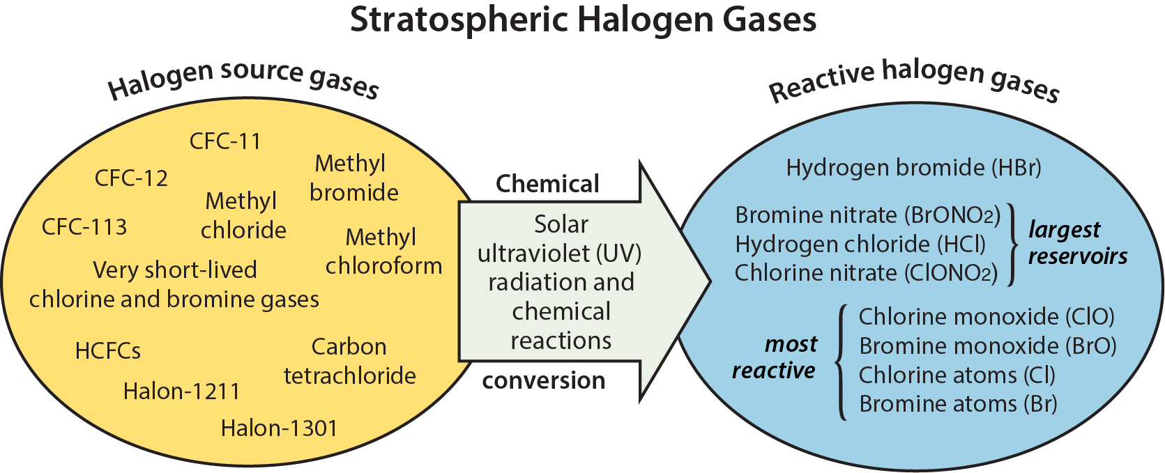
The chlorine- and bromine-containing gases that enter the stratosphere arise from both human activities and natural processes. When exposed to ultraviolet radiation from the Sun, these halogen source gases are converted to more reactive gases that also contain chlorine and bromine. Some reactive gases act as chemical reservoirs which can then be converted into the most reactive gases, namely ClO and BrO. These most reactive gases participate in catalytic reactions that efficiently destroy ozone.
Halogen-containing gases present in the stratosphere can be divided into two groups: halogen source gases and reactive halogen gases (see Figure Q7-1). The source gases, which include ozone-depleting substances (ODSs), are emitted at Earth’s surface by natural processes and by human activities (see Q6). Once in the stratosphere, the halogen source gases chemically convert at different rates to form the reactive halogen gases. The conversion occurs in the stratosphere instead of the troposphere for most gases because solar ultraviolet radiation (a component of sunlight) is more intense in the stratosphere (see Q2). Reactive gases containing the halogens chlorine and bromine lead to the chemical destruction of stratospheric ozone.
Reactive halogen gases. The chemical conversion of halogen source gases, which involves solar ultraviolet radiation and other chemical reactions, produces a number of reactive halogen gases. These reactive gases contain all of the chlorine and bromine atoms originally present in the source gases. The most important reactive chlorine- and bromine-containing gases that form in the stratosphere are shown in Figure Q7-1. Throughout the stratosphere, the most abundant are typically hydrogen chloride (HCl) and chlorine nitrate (ClONO2). These two gases are considered important reservoir gases because, while they do not react directly with ozone, they can be converted to the reactive forms that do chemically destroy ozone. The most reactive forms are chlorine monoxide (ClO) and bromine monoxide (BrO), and chlorine and bromine atoms (Cl and Br). A large fraction of total reactive bromine is generally in the form of BrO, whereas usually only a small fraction of total reactive chlorine is in the form of ClO. The special conditions that occur in the polar regions during winter cause the reservoir gases HCl and ClONO2 to undergo nearly complete conversion to ClO in reactions on polar stratospheric clouds (PSCs) (see Q9).
Reactive chlorine at midlatitudes. Reactive chlorine gases have been observed extensively in the stratosphere using both local and remote measurement techniques. The measurements from space displayed in Figure Q7-2 are representative of how the amounts of chlorine-containing gases change between the surface and the upper stratosphere at middle to high latitudes. Total available chlorine (see red line in Figure Q7-2) is the sum of chlorine contained in halogen source gases (e.g., CFC-11, CFC-12) and in the reactive gases (e.g., HCl, ClONO2, and ClO). Available chlorine is constant to within about 10% from the surface to above 50 km (31 miles) altitude. In the troposphere, total chlorine is contained almost entirely in the source gases described in Figure Q6-1. At higher altitudes, the source gases become a smaller fraction of total available chlorine as they are converted to the reactive chlorine gases. At the highest altitudes, available chlorine is all in the form of reactive chlorine gases.
In the altitude range of the ozone layer at midlatitudes, as shown in Figure Q7-2, the reservoir gases HCl and ClONO2 account for most of the available chlorine. The abundance of ClO, the most reactive gas in ozone depletion, is a small fraction of available chlorine. The low abundance of ClO limits the amount of ozone destruction that occurs outside of polar regions.
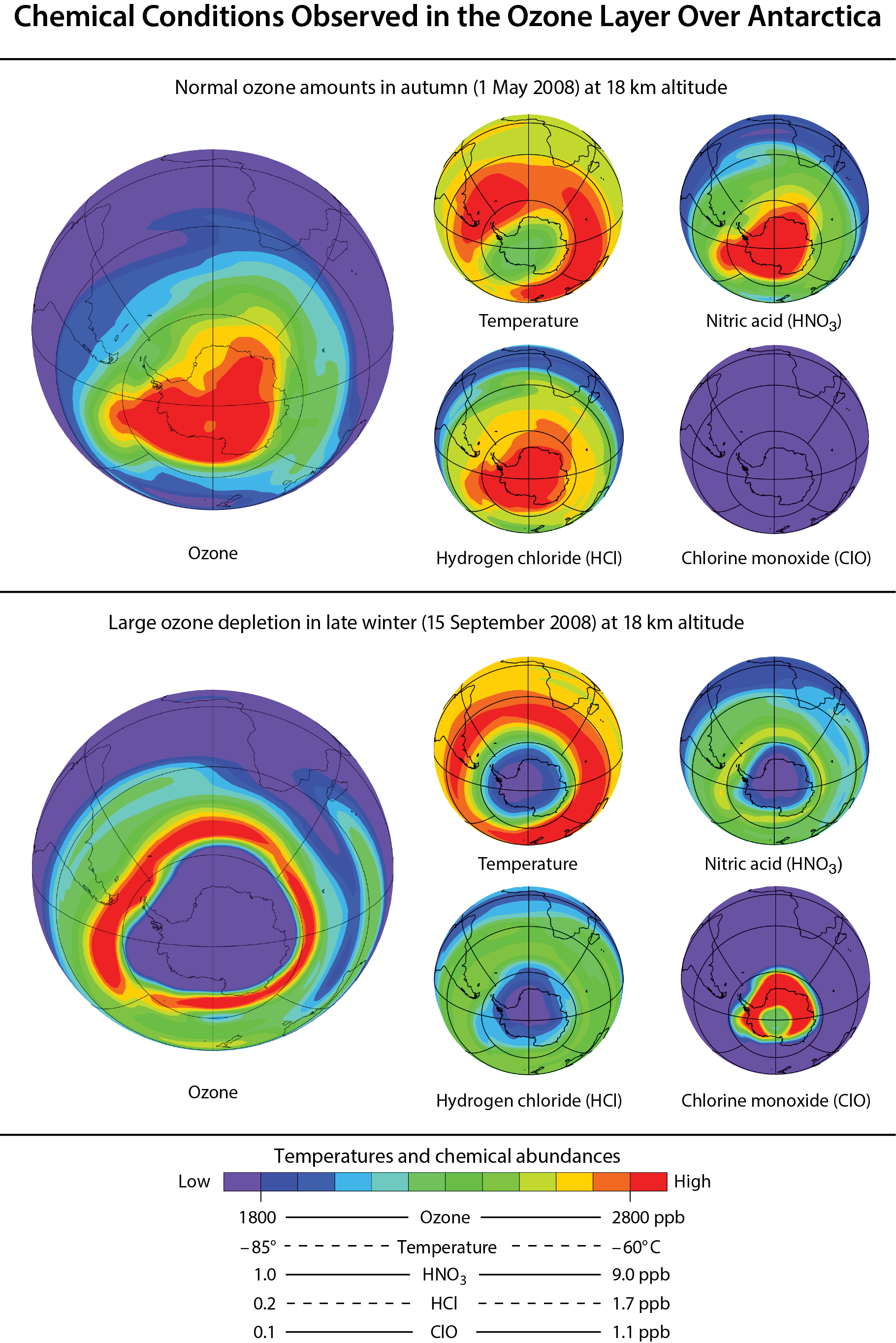
Reactive chlorine in polar regions. Reactive chlorine gases in polar regions undergo large changes between autumn and late winter. Meteorological and chemical conditions in both polar regions are now routinely observed from space in all seasons. Autumn and winter conditions over the Antarctic are contrasted in Figure Q7-3 using seasonal observations made near the center of the ozone layer (about 18 km (11.2 miles) altitude; see Figure Q11-3).
Ozone values are high over the entire Antarctic continent during autumn in the Southern Hemisphere. Temperatures are mid-range, HCl and nitric acid (HNO3) are high, and ClO is very low. High HCl indicates that substantial conversion of halogen source gases has occurred in the stratosphere. In the 1980s and early 1990s, the abundance of reservoir gases HCl and ClONO2 increased substantially in the stratosphere following increased emissions of halogen source gases. HNO3 is an abundant, primarily naturally-occurring stratospheric compound that plays a major role in stratospheric ozone chemistry by both moderating ozone destruction and condensing to form PSCs, thereby enabling conversion of chlorine reservoirs gases to ozone-destroying forms. The low abundance of ClO indicates that little conversion of the reservoir gases occurs in the autumn, thereby limiting catalytic ozone destruction.

(The unit “parts per trillion” is defined in the caption of Figure Q6-1.)
By late winter (September), a remarkable change in the composition of the Antarctic stratosphere has taken place. Low amounts of ozone reflect substantial depletion at 18 km altitude over an area larger than the Antarctic continent. Antarctic ozone holes arise from similar chemical destruction throughout much of the altitude range of the ozone layer (see altitude profile in Figure Q11-3). The meteorological and chemical conditions in late winter, characterized by very low temperatures, very low HCl and HNO3, and very high ClO, are distinctly different from those found in autumn. Low stratospheric temperatures occur during winter, when solar heating is reduced. Low HCl and high ClO reflect the conversion of the reactive halogen reservoir compounds, HCl and ClONO2, to the most reactive form of chlorine, ClO. This conversion occurs selectively in winter on PSCs, which form at very low temperatures (see Q9). Low HNO3 is indicative of its condensation to form PSCs, some of which subsequently descend to lower altitudes through gravitational settling. High ClO abundances generally cause ozone depletion to continue in the Antarctic region until mid-October (spring), when the lowest ozone values usually are observed (see Q10). As temperatures rise at the end of the winter, PSC formation is halted, ClO is converted back into the reservoir species HCl and ClONO2 (see Q9), and ozone destruction is curtailed.
Similar though less dramatic changes in meteorological and chemical conditions are also observed between autumn and late winter in the Arctic, where ozone depletion is less severe than in the Antarctic.
Reactive bromine observations. Fewer measurements are available for reactive bromine gases in the lower stratosphere than for reactive chlorine. This difference arises is in part because of the lower abundance of bromine, which makes quantification of its atmospheric abundance more challenging. The most widely observed bromine gas is BrO, which can be observed from space. Estimates of reactive bromine abundances in the stratosphere are larger than expected from the conversion of the halons and methyl bromide source gases, suggesting that the contribution of the very short-lived bromine-containing gases to reactive bromine must also be significant (see Q6).
(The unit “parts per billion,” abbreviated “ppb,” is used here as a measure of the relative abundance of a substance in dry air: 1 part per billion equals the presence of one molecule of a gas per billion (=109) total air molecules (compare to ppt in Figure Q6-1).)
Reactive gases containing chlorine and bromine destroy stratospheric ozone in “catalytic” cycles made up of two or more separate reactions. As a result, a single chlorine or bromine atom can destroy many thousands of ozone molecules before it leaves the stratosphere. In this way, a small amount of reactive chlorine or bromine has a large impact on the ozone layer. A special situation develops in polar regions in the late winter/early spring season, where large enhancements in the abundance of the most reactive gas, chlorine monoxide, lead to severe ozone depletion.
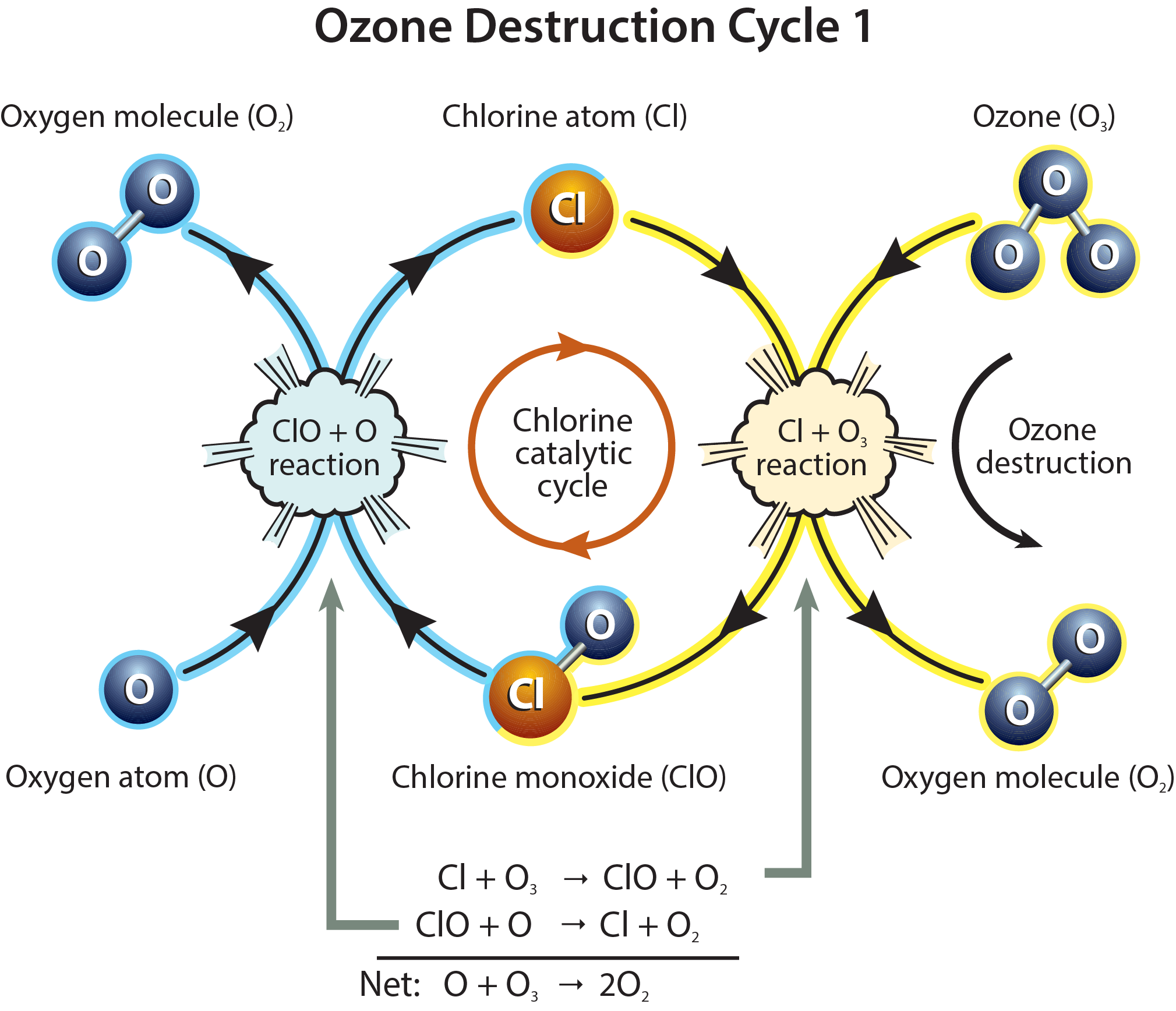
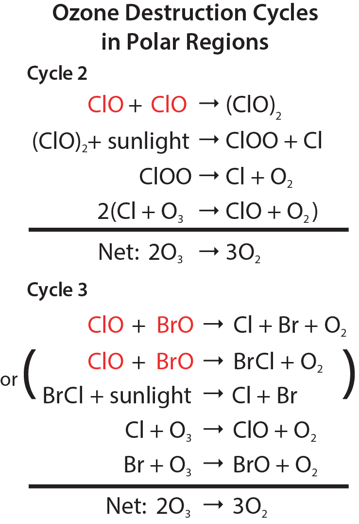
Stratospheric ozone is destroyed by reactions involving reactive halogen gases, which are produced in the chemical conversion of halogen source gases (see Figure Q7-1). The most reactive of these gases are chlorine monoxide (ClO), bromine monoxide (BrO), and chlorine and bromine atoms (Cl and Br). These gases participate in three principal reaction cycles that destroy ozone.
Cycle 1. Ozone destruction Cycle 1 is illustrated in Figure Q8-1. The cycle is made up of two basic reactions: Cl + O3 and ClO + O. The net result of Cycle 1 is to convert one ozone molecule and one oxygen atom into two oxygen molecules. In each cycle, chlorine acts as a catalyst because ClO and Cl react and are reformed. In this way, one Cl atom participates in many cycles, destroying many ozone molecules. For typical stratospheric conditions at middle or low latitudes, a single chlorine atom can destroy thousands of ozone molecules before it happens to react with another gas, breaking the catalytic cycle. During the total time of its stay in the stratosphere, a chlorine atom can thus destroy many thousands of ozone molecules.
Polar Cycles 2 and 3. The abundance of ClO is greatly increased in polar regions during late winter and early spring, relative to other seasons, as a result of reactions on the surfaces of polar stratospheric clouds (see Q7 and Q9). Cycles 2 and 3 (see Figure Q8-2) become the dominant reaction mechanisms for polar ozone loss because of the high abundances of ClO and the relatively low abundance of atomic oxygen (which limits the rate of ozone loss by Cycle 1). Cycle 2 begins with the self-reaction of ClO. Cycle 3, which begins with the reaction of ClO with BrO, has two reaction pathways that produce either Cl and Br or BrCl. The net result of both cycles is to destroy two ozone molecules and create three oxygen molecules. Cycles 2 and 3 account for most of the ozone loss observed in the stratosphere over the Arctic and Antarctic regions in the late winter/early spring season (see Q10 and Q11). At high ClO abundances, the rate of polar ozone destruction can reach 2 to 3% per day.
Sunlight requirement. Sunlight is required to complete and maintain these reaction cycles. Cycle 1 requires ultraviolet (UV) radiation (a component of sunlight) that is strong enough to break apart molecular oxygen into atomic oxygen. Cycle 1 is most important in the stratosphere at altitudes above about 30 km (18.6 miles), where solar UV-C radiation (100 to 280 nanometer (nm) wavelengths) is most intense (see Figure Q2-1).
Cycles 2 and 3 also require sunlight. In the continuous darkness of winter in the polar stratosphere, reaction Cycles 2 and 3 cannot occur. Sunlight is needed to break apart (ClO)2 and BrCl, resulting in abundances of ClO and BrO large enough to drive rapid ozone loss by Cycles 2 and 3. These cycles are most active when sunlight returns to the polar regions in late winter/early spring. Therefore, the greatest destruction of ozone occurs in the partially to fully sunlit periods after midwinter in the polar stratosphere.
Sunlight in the UV-A (315 to 400 nm wavelengths) and visible (400 to 700 nm wavelengths) parts of the spectrum needed in Cycles 2 and 3 is not sufficient to form ozone because this process requires more energetic solar UV-C solar radiation (see Q1 and Q2). In the late winter/early spring, only UV-A and visible solar radiation is present in the polar stratosphere, due to low Sun angles. As a result, ozone destruction by Cycles 2 and 3 in the sunlit polar stratosphere during springtime greatly exceeds ozone production.
Other reactions.. Global abundances of ozone are controlled by many other reactions (see Q1). Reactive hydrogen and reactive nitrogen gases, for example, are involved in catalytic ozone-destruction cycles, similar to those described above, that also take place in the stratosphere. Reactive hydrogen is supplied by the stratospheric decomposition of water (H2O) and methane (CH4). Methane emissions result from both natural sources and human activities. The abundance of stratospheric H2O is controlled by the temperature of the upper tropical troposphere as well as the decomposition of stratospheric CH4. Reactive nitrogen is supplied by the stratospheric decomposition of nitrous oxide (N2O), also emitted by natural sources and human activities. The importance of reactive hydrogen and nitrogen gases in ozone depletion relative to reactive halogen gases is expected to increase in the future because the atmospheric abundances of the reactive halogen gases are decreasing as a result of the Montreal Protocol, while abundances of CH4 and N2O are projected to increase due to various human activities (see Q20).
Ozone-depleting substances are present throughout the stratospheric ozone layer because they are transported great distances by atmospheric air motions. The severe depletion of the Antarctic ozone layer known as the “ozone hole” occurs because of the special meteorological and chemical conditions that exist there and nowhere else on the globe. The very low winter temperatures in the Antarctic stratosphere cause polar stratospheric clouds (PSCs) to form. Special reactions that occur on PSCs, combined with the isolation of polar stratospheric air in the polar vortex, allow chlorine and bromine reactions to produce the ozone hole in Antarctic springtime.
The severe depletion of stratospheric ozone in late winter and early spring in the Antarctic is known as the “ozone hole” (see Q10). The ozone hole appears over Antarctica because meteorological and chemical conditions unique to this region increase the effectiveness of ozone destruction by reactive halogen gases (see Q7 and Q8). In addition to a large abundance of these reactive gases, the formation of the Antarctic ozone hole requires temperatures low enough to form polar stratospheric clouds (PSCs), isolation from air in other stratospheric regions, and sunlight (see Q8).
Distribution of halogen gases. Halogen source gases that are emitted at Earth’s surface and have lifetimes longer than about 1 year (see Table Q6-1) are present in comparable abundances throughout the stratosphere in both hemispheres, even though most of the emissions occur in the Northern Hemisphere. The abundances are comparable because most long-lived source gases have no significant natural removal processes in the lower atmosphere, and because winds and convection redistribute and mix air efficiently throughout the troposphere on the timescale of weeks to months. Halogen gases (in the form of source gases and some reactive products) enter the stratosphere primarily from the tropical upper troposphere. Stratospheric air motions then transport these gases upward and toward the pole in both hemispheres.
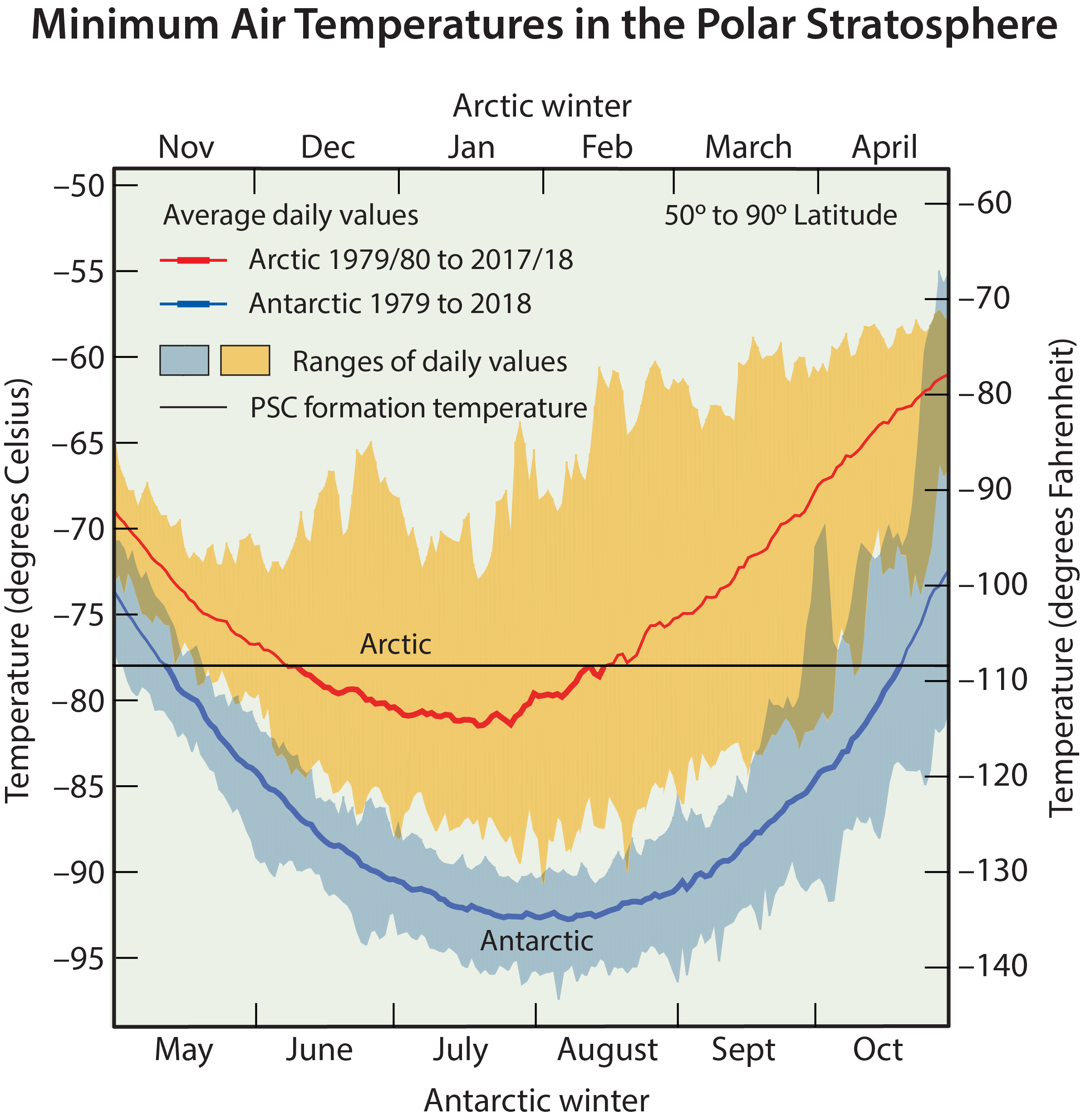
Low polar temperatures. The severe ozone destruction that leads to the ozone hole requires low temperatures to be present over a range of stratospheric altitudes, over large geographical regions, and for extended time periods. Low temperatures are important because they allow liquid and solid PSCs to form. Reactions on the surfaces of these PSCs initiate a remarkable increase in the most reactive chlorine gas, chlorine monoxide (ClO) (see below as well as Q7 and Q8). Stratospheric temperatures are lowest in the polar regions in winter. In the Antarctic winter, minimum daily temperatures are generally much lower and less variable than those in the Arctic winter (see Figure Q9-1). Antarctic temperatures also remain below PSC formation temperatures for much longer periods during winter. These and other meteorological differences occur because of variations between the hemispheres in the distributions of land, ocean, and mountains at middle and high latitudes. As a consequence, winter temperatures are low enough for PSCs to form somewhere in the Antarctic for nearly the entire winter (about 5 months), and only for limited periods (10–60 days) in the Arctic for most winters.
Isolated conditions. Stratospheric air in the polar regions is relatively isolated for long periods in the winter months. The isolation is provided by strong winds that encircle the poles during winter, forming a polar vortex, which prevents substantial transport and mixing of air into or out of the polar stratosphere. This circulation strengthens in winter as stratospheric temperatures decrease. The Southern Hemisphere polar vortex circulation tends to be stronger than that in the Northern Hemisphere because northern polar latitudes have more land and mountainous regions than southern polar latitudes. This situation leads to more meteorological disturbances in the Northern Hemisphere, which increase the mixing in of air from lower latitudes that warms the Arctic stratosphere. Since winter temperatures are lower in the Southern than in the Northern Hemisphere polar stratosphere, the isolation of air in the polar vortex is much more effective in the Antarctic than in the Arctic. Once temperatures drop low enough, PSCs form within the polar vortex and induce chemical changes such as an increase in the abundance of ClO (see Q8) that are preserved for many weeks to months due to the isolation of polar air.
Polar stratospheric clouds (PSCs). Reactions on the surfaces of liquid and solid PSCs can substantially increase the relative abundances of the most reactive chlorine gases. These reactions convert the reservoir forms of reactive chlorine gases, chlorine nitrate (ClONO2) and hydrogen chloride (HCl), to the most reactive form, ClO (see Figure Q7-3). The abundance of ClO increases from a small fraction of available reactive chlorine to comprise nearly all chlorine that is available. With increased ClO, the catalytic cycles involving ClO and BrO become active in the chemical destruction of ozone whenever sunlight is available (see Q8).
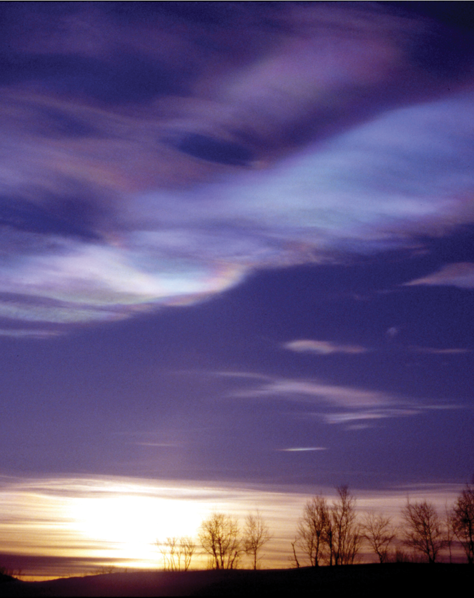
Different types of liquid and solid PSC particles form when stratospheric temperatures fall below about −78°C (−108°F) in polar regions (see Figure Q9-1). As a result, PSCs are often found over large areas of the winter polar regions and over significant altitude ranges, with significantly larger regions and for longer time periods in the Antarctic than in the Arctic. The most common type of PSC forms from nitric acid (HNO3) and water condensing on pre-existing liquid sulfuric acid-containing particles. Some of these particles freeze to form solid particles. At even lower temperatures (−85°C or −121°F), water condenses to form ice particles. PSC particles grow large enough and are numerous enough that cloud-like features can be observed from the ground under certain conditions, particularly when the Sun is near the horizon (see Figure Q9-2). PSCs are often found near mountain ranges in polar regions because the motion of air over the mountains can cause localized cooling in the stratosphere, which increases condensation of water and HNO3.
When average temperatures begin increasing in late winter, PSCs form less frequently, which slows down the production of ClO by conversion reactions throughout the polar region. Without continued production, the abundance of ClO decreases as other chemical reactions re-form the reservoir gases, ClONO2 and HCl. When temperatures rise above PSC formation thresholds, usually sometime between late January and early March in the Arctic and by mid-October in the Antarctic (see Figure Q9-1), the most intense period of ozone depletion ends.
Nitric acid and water removal. Once formed, the largest PSC particles fall to lower altitudes because of gravity. The largest particles can descend several kilometers or more in the stratosphere within a few days during the low-temperature winter/ spring period. Because PSCs often contain a significant fraction of available HNO3, their descent removes HNO3 from regions of the ozone layer. This process is called denitrification of the stratosphere. Because HNO3 is a source for nitrogen oxides (NOx) in the stratosphere, denitrification removes the NOx available for converting the highly reactive chlorine gas ClO back into the reservoir gas ClONO2. As a result, ClO remains chemically active for a longer period, thereby increasing chemical ozone destruction. Significant denitrification occurs each winter in the Antarctic and only for occasional winters in the Arctic, because PSC formation temperatures must be sustained over an extensive altitude region and time period to lead to denitrification (see Figure Q9-1).
Ice particles form at temperatures that are a few degrees lower than those required for PSC formation from HNO3. If ice particles grow large enough, they can fall several kilometers due to gravity. As a result, a significant fraction of water vapor can be removed from regions of the ozone layer over the course of a winter. This process is called dehydration of the stratosphere. Because of the very low temperatures required to form ice, dehydration is common in the Antarctic and rare in the Arctic. The removal of water vapor does not directly affect the catalytic reactions that destroy ozone. Dehydration indirectly affects ozone destruction by suppressing PSC formation later in winter, which reduces the production of ClO by PSC reactions.
Discovering the role of PSCs. Ground-based observations of PSCs were available many decades before the role of PSCs in polar ozone destruction was recognized. The geographical and altitude extent of PSCs in both polar regions was not known fully until PSCs were observed by a satellite instrument in the late 1970s. The role of PSC particles in converting reactive chlorine gases to ClO was not understood until after the discovery of the Antarctic ozone hole in 1985. Our understanding of the chemical role of PSC particles developed from laboratory studies of their surface reactivity, computer modeling studies of polar stratospheric chemistry, and measurements that directly sampled particles and reactive chlorine gases, such as ClO, in the polar stratosphere.
Stratospheric ozone depletion
Severe depletion of the Antarctic ozone layer was first reported in the mid-1980s. Antarctic ozone depletion is seasonal, occurring primarily in late winter and early spring (August–November). Peak depletion occurs in early October when ozone is often completely destroyed over a range of stratospheric altitudes, thereby reducing total ozone by as much as two-thirds at some locations. This severe depletion creates the “ozone hole” apparent in images of Antarctic total ozone acquired using satellite instruments. In most years the maximum area of the ozone hole far exceeds the size of the Antarctic continent.
The severe depletion of Antarctic ozone, known as the “ozone hole”, was first reported in the mid-1980s (see box in Q9). The depletion is attributable to chemical destruction by reactive halogen gases (see Q7 and Q8), which increased everywhere in the stratosphere in the latter half of the 20th century (see Q15). Conditions in the Antarctic winter and early spring stratosphere enhance ozone depletion because of (1) the long periods of extremely low temperatures, which cause polar stratospheric clouds (PSCs) to form; (2) the large abundance of reactive halogen gases produced in reactions on PSCs; and (3) the isolation of stratospheric air, which allows time for chemical destruction processes to occur. The severity of Antarctic ozone depletion as well as long-term changes can be seen using satellite observations of total ozone and ozone altitude profiles.
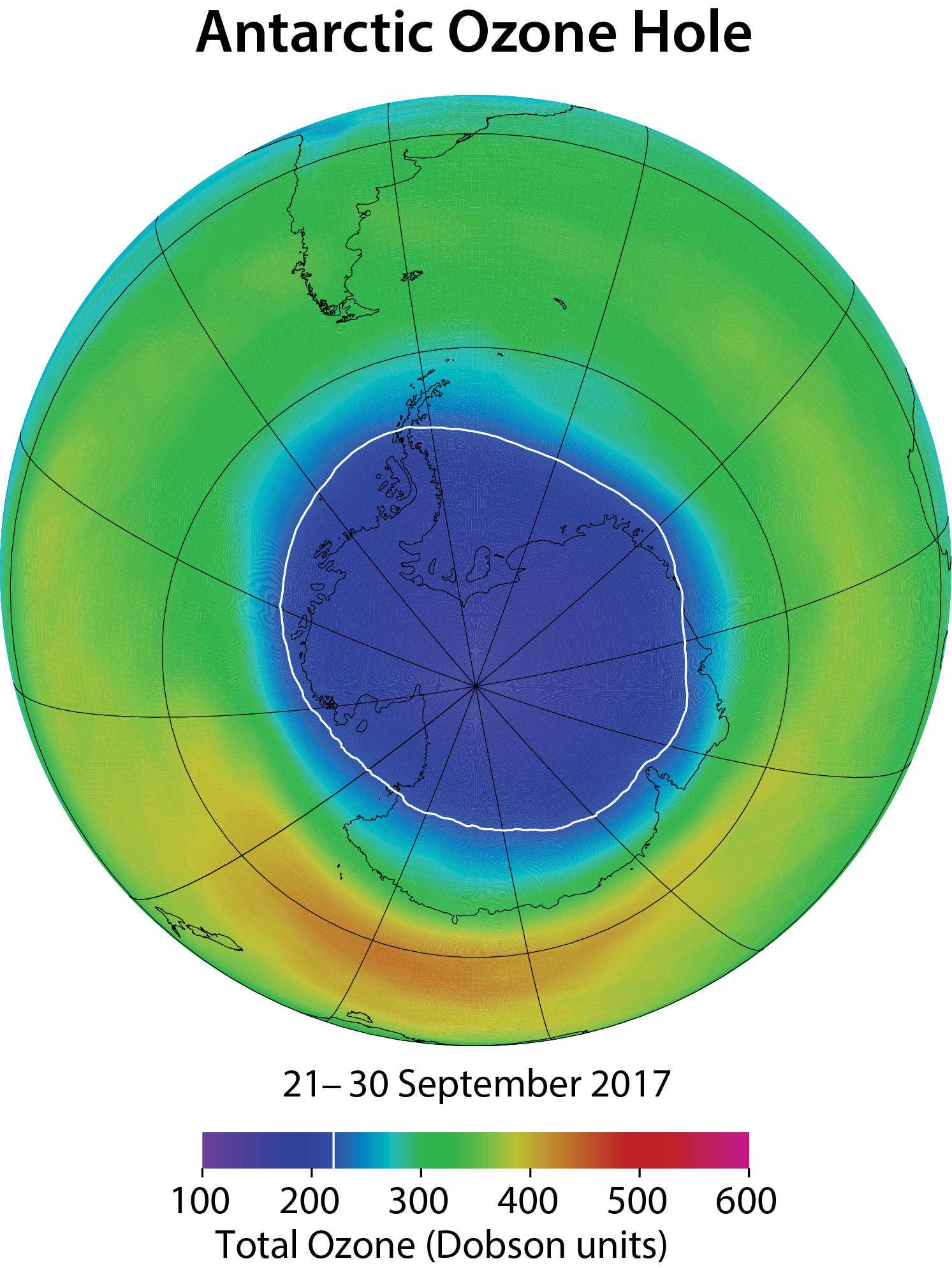
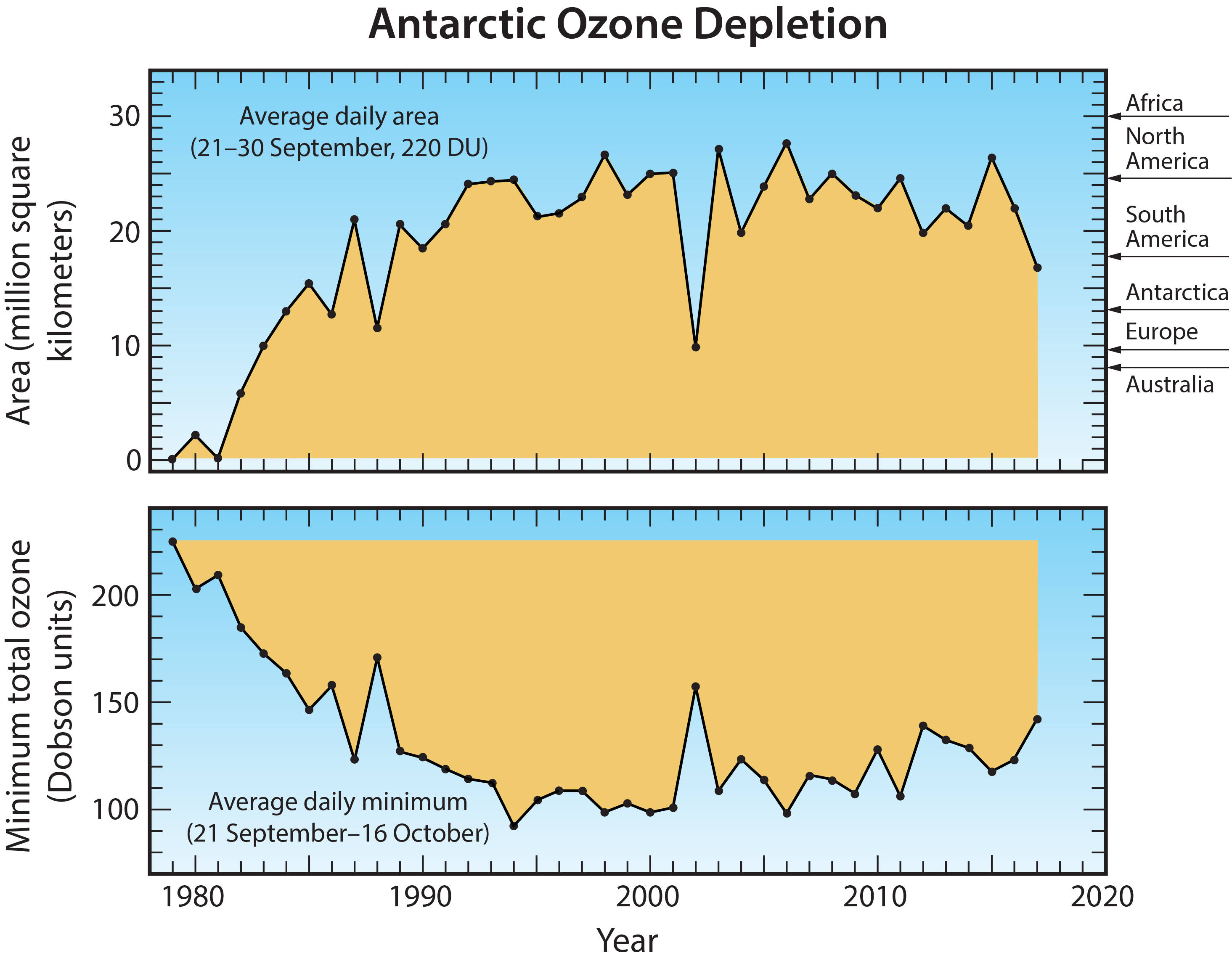
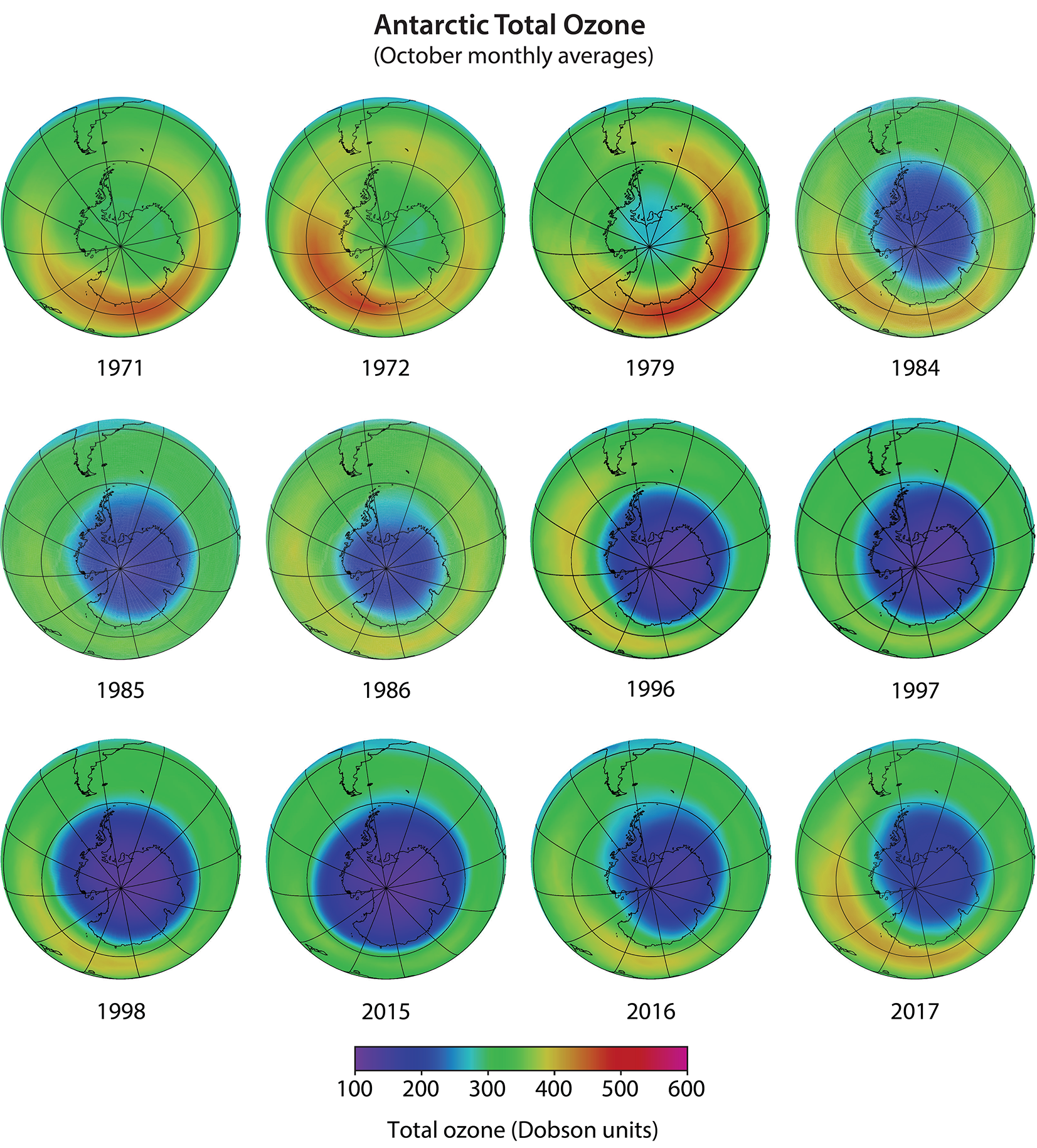
Antarctic ozone hole. The most widely used images of Antarctic ozone depletion are derived from measurements of total ozone made with satellite instruments. A map of Antarctic early spring measurements shows a large region centered near the South Pole in which total ozone is highly depleted (see Figure Q10-1). This region has come to be called the “ozone hole” because of the near-circular contours of low ozone values in the maps. The area of the ozone hole is defined here as the geographical region within the 220-Dobson unit (DU) contour in total ozone maps (see white line in Figure Q10-1) averaged between 21–30 September for a given year. The area reached a maximum of 28 million square km (about 11 million square miles) in 2006, which is more than twice the area of the Antarctic continent (see Figure Q10-2). Minimum values of total ozone inside the ozone hole averaged in late September to mid-October are near 120 DU, which is nearly two-thirds below springtime values of about 350 DU observed in the early 1970s (see Figures Q10-3 and Q11-1). Low total ozone inside the ozone hole contrasts strongly with the distribution of much larger values outside the ozone hole. This common feature can be seen in Figure Q10-1, where a crescent-shaped region with values around 400 DU surrounds a significant portion of the ozone hole in September 2017, and reveals the edge of the polar vortex that acts as a barrier to the transport of ozone-rich midlatitude air into the polar region (see Q9).
Altitude profiles of Antarctic ozone. The low total ozone values within the ozone hole are caused by nearly complete removal of ozone in the lower stratosphere. Balloon-borne instruments (see Q4) demonstrate that this depletion occurs within the ozone layer, the altitude region that normally contains the highest abundances of ozone. At geographic locations with the lowest total ozone values, balloon measurements show that the chemical destruction of ozone has often been complete over an altitude region of up to several kilometers. For example, in the ozone profile over South Pole, Antarctica on 9 October 2006 (see red line in left panel of Figure Q11-3), ozone abundances are essentially zero over the altitude region of 14 to 21 km. The lowest winter temperatures and highest reactive chlorine (ClO) abundances occur in this altitude region (see Figure Q7-3). The differences in the average South Pole ozone profiles between the decade 1962–1971 and the years 1990–2018 in Figure Q11-3 show how reactive halogen gases have dramatically altered the ozone layer. In the 1960s, a normal ozone layer is clearly evident in the October average profile, with a peak near 16 km altitude. In the 1990–2018 average profile, a broad minimum centered near 16 km now occurs, with ozone values reduced by up to 90% relative to normal values.
Long-term total ozone changes. Prior to 1960, the amount of reactive halogen gases in the stratosphere was insufficient to cause significant chemical loss of Antarctic ozone. Ground-based observations show that the steady decline in total ozone over the Halley Bay, Antarctic research station (76°S) (see box in Q9) during each October first became apparent in the early 1970s.
Satellite observations reveal that in 1979, total ozone during October near the South Pole was slightly lower than found at other high southerly latitudes (see Figure 10-3). Computer model simulations indicate Antarctic ozone depletion actually began in the early 1960s. Until the early 1980s, total ozone depletion was not large enough to result in minimum values falling below the 220 DU threshold that is now commonly used to denote the boundary of the ozone hole (see Figure Q10-1). Starting in the mid-1980s, a region of total ozone well below 220 DU centered over the South Pole became apparent in satellite maps of October total ozone (see Figure Q10-3). Observations of total ozone from satellite instruments can be used in multiple ways to examine how ozone depletion has changed in the Antarctic region over the past 50 years, including:
First, ozone hole areas displayed in Figure Q10-2 show that depletion increased after 1980, then became fairly stable in the 1990s, 2000s, and into the mid-2010s, often reaching an area of 24 million square km (about the size of North America). An exception is the unexpectedly low depletion in 2002, which is explained in the box at the end of this Question. The ozone hole area was larger in 2015, compared to 2014 and 2016, due to the presence of an unusually cold and stable polar vortex in 2015 as well as an increase in stratospheric particles due to the Calbuco volcanic eruption in southern Chile during April 2015.
Second, minimum Antarctic ozone amounts displayed in Figure Q10-2 show that the severity of the depletion increased beginning around 1980 along with the rise in the ozone hole area. Fairly constant minimum values of total ozone, near 110 DU, were observed in the 1990s and 2000s, with the exception of 2002. There is some indication of an increase in the minimum value of total ozone since the early 2010s.
Third, total ozone maps over the Antarctic and surrounding regions show how the ozone hole has developed over time in Figure Q10-3. October averages show the absence of an ozone hole in the 1970s, the extent of the ozone hole around the time of its discovery in 1985 (see box in Q9), and the annual occurrence throughout the 1990s and 2010s.
Fourth, values of total ozone averaged poleward of 63°S for each October show how total ozone has changed in the Antarctic region in Figure Q11-1. After decreasing steeply in the early years of the ozone hole, polar-cap averages of total ozone are now approximately 30% smaller than those in pre-ozone hole years (1970–1982). These Antarctic-region ozone values exhibit larger year-to-year variability than the other ozone measures noted above because this average includes areas outside the ozone hole. Increased year-to-year variability in Antarctic-region ozone is evident over the past decade. As noted above, the exceptionally low value of total ozone in 2015 is attributed in part to the effects of the Calbuco volcanic eruption, whereas the 2017 ozone hole was less extensive than prior years due to unusual meteorological conditions in the Southern Hemisphere. The maps in Figure Q10-3 show how the maximum in total ozone surrounding the ozone hole each year has also diminished over the last four decades, adding to the decreases noted in Figure Q11-1.
Disappearance of the Antarctic ozone hole in spring. The severe depletion of Antarctic ozone occurs in the late winter/early spring season. In austral spring (mid-October), temperatures in the polar lower stratosphere increase (see Figure Q9-1), stopping the formation of PSCs and production of ClO and, consequently, the most effective chemical cycles that destroy ozone (see Q8). The polar vortex breaks down, ending the wintertime isolation of high-latitude air and increasing the exchange of air between the Antarctic stratosphere and lower latitudes. This allows substantial amounts of ozone-rich air to be transported poleward, where it displaces or mixes with air depleted in ozone. The midlatitude air also contains higher abundances of nitrogen oxide gases (NOx), which help convert the most reactive chlorine gases (ClO) back into the chlorine reservoir gas ClONO2 (see Q7 and Q9). As a result of these large-scale transport and mixing processes, the ozone hole typically disappears by mid-December.

Yes, significant depletion of the Arctic ozone layer now occurs in most years in the late winter and early spring period (January–March). However, Arctic ozone depletion is less severe than that observed in the Antarctic and exhibits larger year-to-year differences as a consequence of the highly variable meteorological conditions found in the Arctic polar stratosphere. Even the most severe Arctic ozone depletion does not lead to total ozone amounts as low as those seen in the Antarctic, because Arctic ozone abundances during early winter before the onset of ozone depletion are much larger than those in the Antarctic. Consequently, an extensive and recurrent “ozone hole”, as found in the Antarctic stratosphere, does not occur in the Arctic.
Significant depletion of ozone has been observed in the Arctic stratosphere in recent decades. The depletion is attributable to chemical destruction by reactive halogen gases (see Q8), which increased in the stratosphere in the latter half of the 20th century (see Q15). Arctic depletion also occurs in the late winter/ early spring period (January–March), however over a somewhat shorter period than in the Antarctic (July–October). Similar to the Antarctic (see Q10), Arctic ozone depletion occurs because of (1) periods of very low temperatures, which lead to the formation of polar stratospheric clouds (PSCs); (2) the large abundance of reactive halogen gases produced in reactions on PSCs; and (3) the isolation of polar stratospheric air, which allows time for chemical destruction processes to occur.
Arctic ozone depletion is much less than that observed each Antarctic winter/spring season. Extensive and recurrent ozone holes as found in the Antarctic stratosphere do not occur in the Arctic. Stratospheric ozone abundances during early winter, before the onset of ozone depletion, are naturally higher in the Arctic than in the Antarctic because transport of ozone from its source region in the tropics to higher latitudes is more vigorous in the Northern Hemisphere. Furthermore, ozone depletion is limited because, in comparison to Antarctic conditions, average temperatures in the Arctic stratosphere are always significantly higher (see Figure Q9-1) and the isolation of polar stratospheric air is less effective (see Q9). These differences occur because northern polar latitudes have more land and mountainous regions than southern polar latitudes (compare Figures Q10-3 and Q11-2 at 60° latitude), which creates more meteorological disturbances that warm the Arctic stratosphere (see box in Q10). Consequently, the extent and timing of Arctic ozone depletion varies considerably from year to year. In a few of the Arctic winters for the years shown in Figure Q11-1, PSCs did not form because temperatures were never sufficiently low. Ozone depletion in some winter/spring seasons occurs over many weeks, in others only for brief early or late periods, and in some not at all.
Long-term total ozone changes. Two important ways in which satellite observations can be used are to examine the average total ozone abundances in the Arctic region for the last half century and to contrast these values with Antarctic abundances:
First, total ozone averaged poleward of 63°N for each March shows how total ozone has changed in the Arctic (see Figure Q11-1). The seasonal poleward and downward transport of ozone-rich air is naturally stronger in the Northern Hemisphere. As a result, total ozone values at the beginning of each winter season in the Arctic are considerably higher than those in the Antarctic. Before ozone depletion begins, normal Arctic values are close to 450 DU while Antarctic values are close to 330 DU. Decreases from pre-ozone-hole average values (1970–1982) were observed in the Arctic by the mid-1980s, when larger changes were already occurring in the Antarctic. The decreases in total ozone in the Arctic are generally much smaller than those found in the Antarctic and lead to total ozone values that are typically about 10 to 20% below normal. Maximum decreases in total ozone of about 30% observed in March 1997 and 2011 for considerable regions of the Arctic (see Figure Q11-2) are the most comparable to Antarctic depletion. In both of these Arctic winters, meteorological conditions inhibited transport of ozone-rich air to high latitudes, and in 2011 persistently low temperatures facilitated severe chemical depletion of ozone by reactive halogens (see Q8).
Overall, Arctic total ozone values exhibit larger year-to-year variability than those in the Antarctic. Ozone differences from the 1970–1982 average value are due to a combination of chemical destruction by halogens and meteorological (natural) variations. In the last quarter century, these two aspects have contributed about equally to observed ozone changes. The amount of chemical destruction depends in large part on stratospheric temperatures. Meteorological conditions determine how well Arctic stratospheric air is isolated from ozone-rich air at lower latitudes and also influence the extent and persistence of low temperatures.
Second, total ozone maps over the Arctic and surrounding regions (see Figure Q11-2) show year-to-year changes in total ozone during March. In the 1970s, total ozone values were near 450 DU when averaged over the Arctic region in March. Beginning in the 1990s and continuing into the mid-2010s, values above 450 DU were increasingly absent from the March average maps. A comparison of the maps in the 1970s and early to mid-2010s, for example, shows a striking reduction of total ozone throughout the Arctic region. The large geographical extent of low total ozone in the maps of March 1997 and March 2011 represent exceptional events in the Arctic observational record of the last four decades as noted above in the discussion of Figure Q11-1. The high values of total ozone observed throughout the Arctic during March 2018 followed a meteorological warming event in late February that disrupted the polar vortex circulation and transported large amounts of ozone to high northerly latitudes. The large-scale differences between Arctic ozone distributions observed in March 2011, 2014, and 2018 are a prime example of the influence of meteorology in driving year-to-year variations in Arctic ozone depletion.
Altitude profiles of Arctic ozone. Arctic ozone is measured using a variety of instruments (see Q4), as in the Antarctic, to document daily to seasonal changes within the ozone layer. Spring Arctic and Antarctic balloon-borne measurements are shown in Figure Q11-3. Arctic profiles were obtained from the Ny-Ålesund research station at 79°N. For 1990–2018, the March average reveals a substantial ozone layer, contrasting sharply with the severely depleted Antarctic ozone layer in the October average over a similar time period. This contrast further demonstrates how higher stratospheric temperatures and more variable meteorology have protected the Arctic ozone layer from the greater ozone losses that occur in the Antarctic, despite similar abundances of reactive halogen gases (see Q7) in the two regions.
The Arctic profiles shown in Figure Q11-3 for 29 March 1996 and 1 April 2011 are two of the most severely depleted in the 30-year record from Ny-Ålesund. Although significant, the depletion during both events is smaller in comparison to that routinely observed in the Antarctic, such as in the profile from 9 October 2006. In the Antarctic stratosphere, near-complete depletion of ozone over many kilometers in altitude and over areas almost as large as North America is a common occurrence. Ozone depletion of this magnitude has never been observed in the Arctic stratosphere.
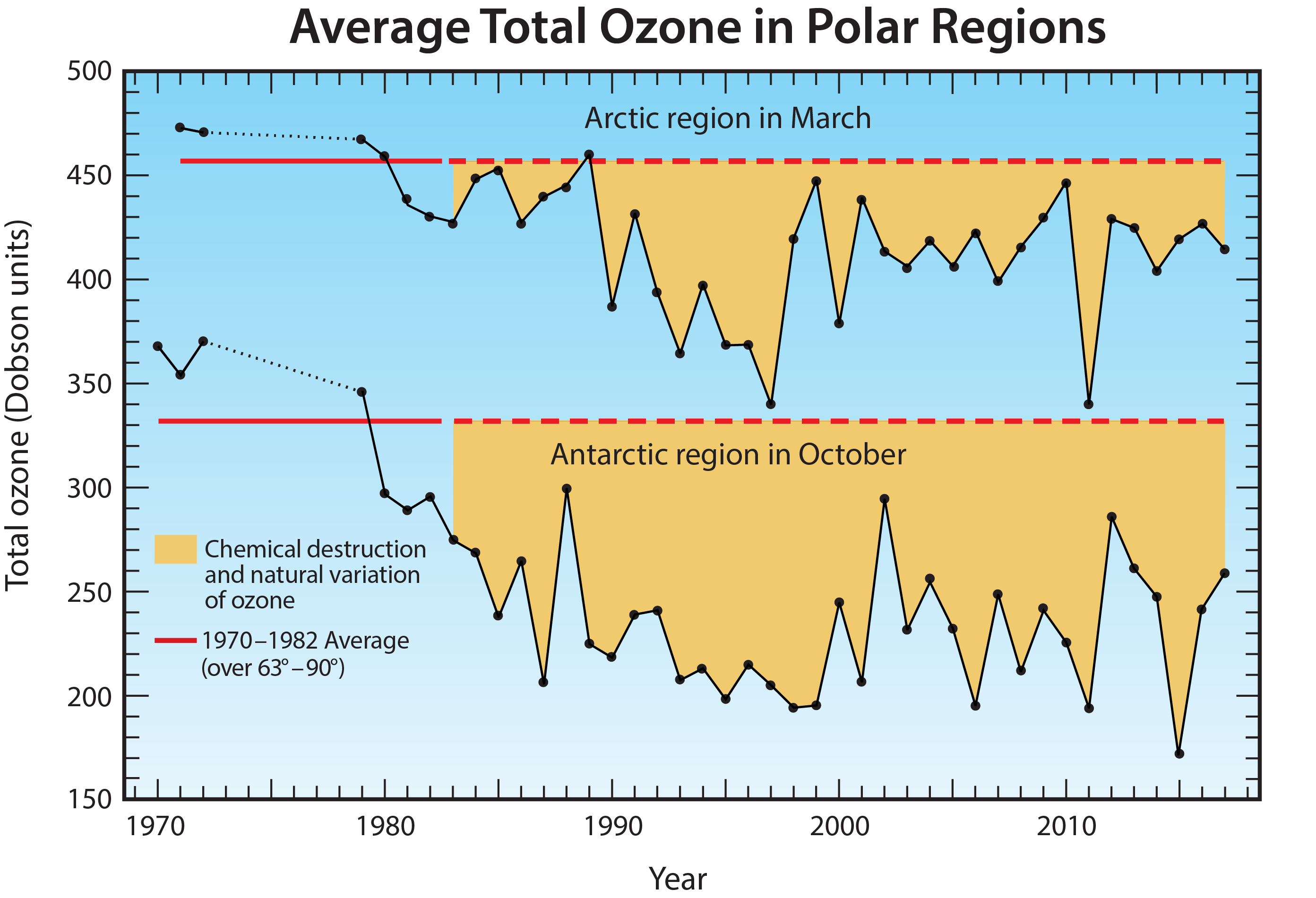
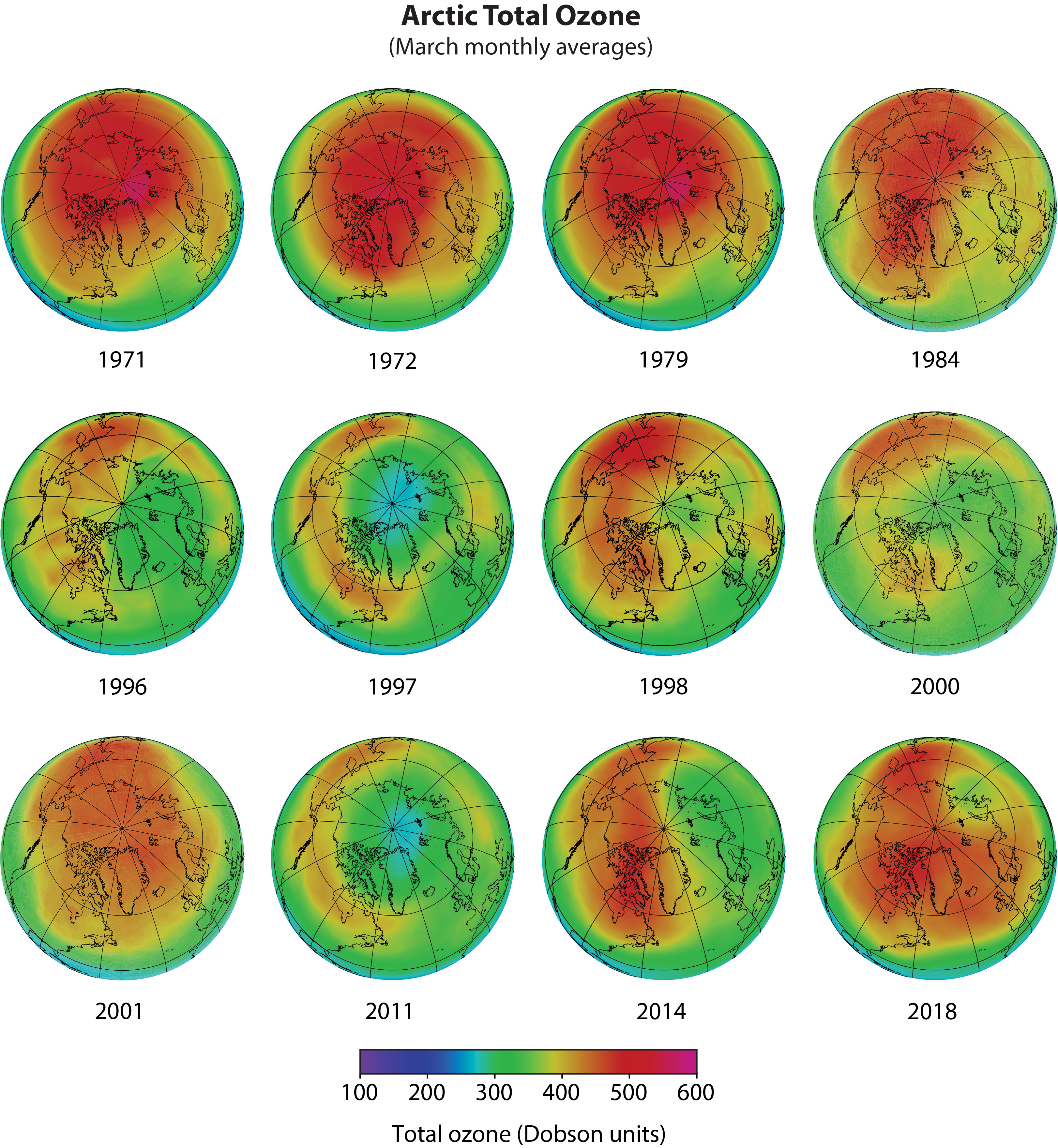
Restoring ozone in spring. As in the Antarctic, ozone depletion in the Arctic is largest in the late winter/early spring season. In spring, temperatures in the polar lower stratosphere increase (see Figure Q9-1), halting the formation of PSCs, the production of ClO, and the chemical cycles that destroy ozone. The breakdown of the polar vortex ends the isolation of air in the high-latitude region, allowing more ozone-rich air to be transported poleward where it displaces or mixes with air in which ozone may have been depleted. As a result of these large-scale transport and mixing processes, any ozone depletion at high northern latitudes typically disappears by April or earlier.
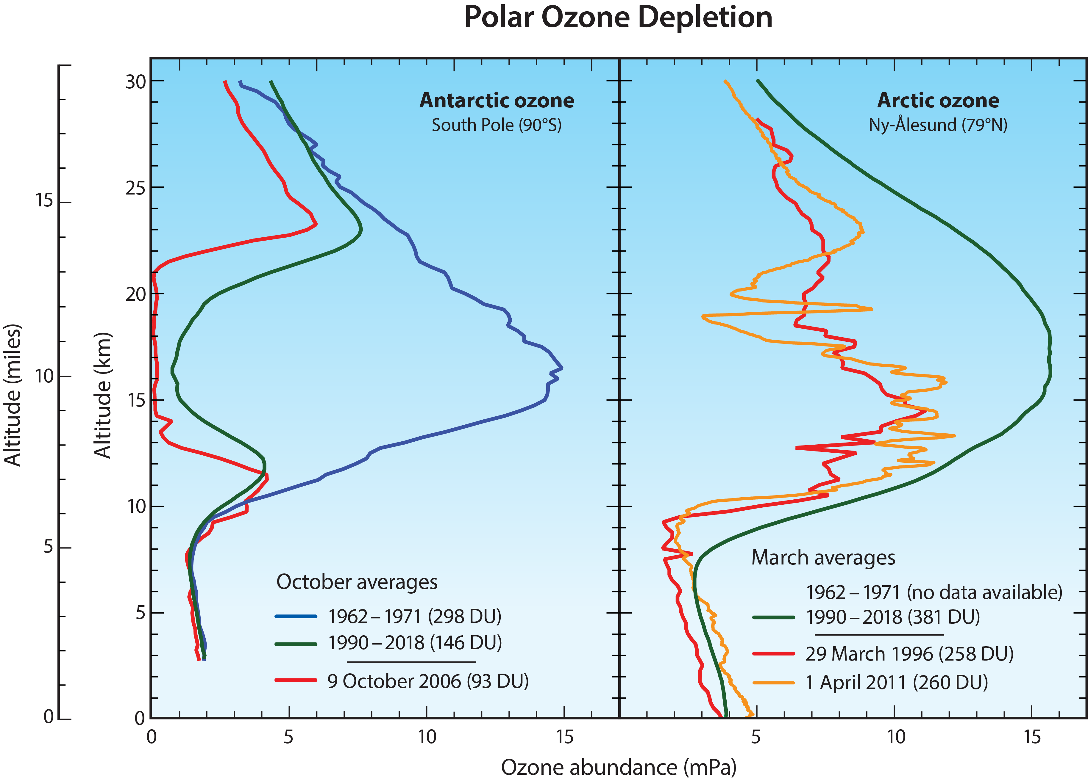
The abundance of globally averaged total ozone is now about 2–3% below the amount present during 1964–1980. The abundance of global total ozone declined steadily throughout the 1980s due to the increases in reactive halogen gases in the stratosphere resulting from human activities. In the early 1990s, global total ozone was depleted by 5% relative to the 1964–1980 average, the maximum depletion observed during the modern instrument era. In both hemispheres, total ozone depletion is small near the equator and increases toward the poles. The larger depletion at higher latitudes is due, in part, to the late winter/early spring destruction of ozone that occurs in polar regions, particularly in Antarctica.
Global total ozone started decreasing in the 1980s (see Figure Q12-1) due to the rise in stratospheric halogens that result from human activities (see Figure Q15-1). Most of the depletion has occurred in the stratospheric ozone layer, where most ozone resides (see Figure Q1-2). By the early 1990s, total ozone was 5% lower than the 1964–1980 average. Ozone depletion subsequently diminished, so that by 2010 globally averaged ozone was 2-3% less than the 1964–1980 average. The observations shown in Figure Q12-1 have been smoothed to remove regular variations in ozone due to natural seasonal effects and year-to-year changes in atmospheric circulation (see Q13). Over the past few years, observed global ozone has been about 2.2% lower than the 1964-1980 average.
The observed global ozone depletion in the past four decades is attributable to increases in reactive halogen gases in the stratosphere (see Q13). The lowest global total ozone values since 1980 have occurred in the years following the volcanic eruption of Mount Pinatubo in 1991, which temporarily increased the number of sulfuric acid-containing particles throughout the stratosphere. These particles significantly increased the effectiveness of reactive halogen gases in destroying ozone (see Q13) and, thereby, increased global ozone depletion by about 2% for several years following the eruption.
Polar regions. Observed total ozone depletion varies significantly with latitude across the globe (see Figure Q12-1). The largest reductions occur at high southern latitudes as a result of the severe ozone loss over Antarctica each late winter/early spring period (see Q9 and Q10). The next largest losses are observed in the high latitudes of the Northern Hemisphere, caused in part by winter losses over the Arctic in some years (see Q11). Although the depletion of ozone in polar regions is larger than at lower latitudes, the contribution of polar ozone loss to globally averaged depletion is limited by the smaller geographical area of high-latitude regions. Latitudes poleward of 60° account for only about 13% of Earth’s surface.
Midlatitude regions. Ozone depletion is also observed at mid-latitudes. In comparison with the 1964–1980 average amounts, total ozone averaged for 2012–2016 is about 3% lower in northern midlatitudes (35°N–60°N) and about 5.5% lower at southern midlatitudes (35°S–60°S). Midlatitude depletion has two contribu ting factors. First, ozone-depleted air over both polar regions is dispersed away from the poles during and after each winter/spring period, thereby reducing average ozone at midlatitudes. Second, chemical destruction occurring at mid-latitudes contributes to observed depletion in these regions. Ozone depletion at midlatitudes is much smaller than in polar regions (see Q20) because the amount of reactive halogen gases is lower and the seasonal increase of ClO, the most reactive halogen gas, does not occur.
Tropical region. Total ozone in the tropics (20°N–20°S latitude) has been only weakly affected by chemical depletion. In the tropical lower stratosphere, air is transported from the lower atmosphere (troposphere) over about an 18-month period. As a result, the fraction of ozone-depleting substances (ODSs) converted to reactive halogen gases is still very small. With little reactive halogen available, total ozone depletion in this region is also very small. In addition, net ozone production occurs in the tropics because of high average amounts of solar ultraviolet radiation. In contrast, stratospheric air in polar regions has been in the stratosphere for an average of 4 to 7 years, allowing time for significant conversion of ODSs to reactive halogen gases (see Figure Q5-1). These systematic differences in stratospheric air are a consequence of large-scale atmospheric transport: air enters the stratosphere in the tropics, moves poleward in both hemispheres, and then descends and ultimately returns to the troposphere in the middle to high latitudes.
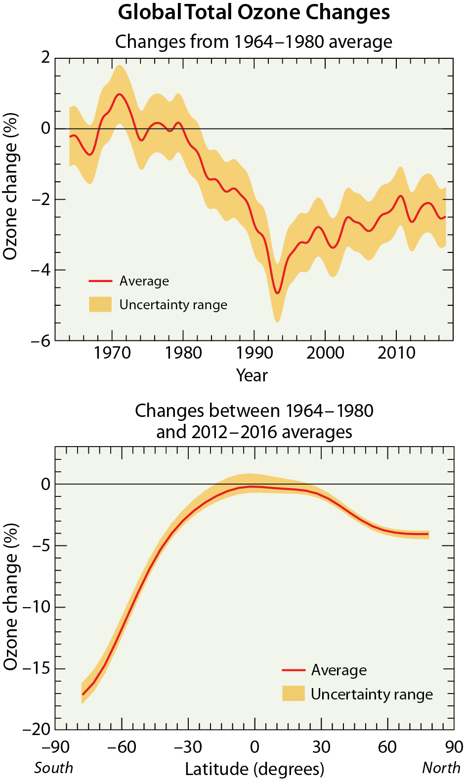
Yes, factors such as changes in solar radiation and the formation of stratospheric aerosol particles after explosive volcanic eruptions do influence the ozone layer. Global ozone abundances vary by 1–2% between the maximum and minimum of the 11-year solar cycle. The abundance of global ozone decreased by about 2% for a few years after the June 1991 eruption of Mount Pinatubo, due to volcanic enhancement of stratospheric sulfate aerosols. However, neither factor can explain the observed decrease in global total ozone or the severe ozone depletion observed in polar regions over the past half century. The primary influence on long-term changes in total global ozone is the abundance of stratospheric halogens.
Changes in solar radiation and increases in stratospheric aerosols (small particles) from volcanic eruptions both affect the abundance of stratospheric ozone. Global total ozone in the early 1990s decreased by about 5% when compared to pre-1980 values, and is now about 2-3% below the 1964–1980 average value (see Q12). The long-term depletion of ozone is primarily attributed to increases in reactive halogen gases, with additional depletion in the early 1990s associated with the volcanic eruption of Mount Pinatubo. Equivalent effective stratospheric chlorine (EESC) is often used as a measure of the potential of reactive halogen gases to deplete ozone (see definition in Q15). Comparisons of the long-term changes in solar radiation, stratospheric volcanic aerosol, and EESC are useful in evaluating the contribution of these factors to long-term changes in total ozone.
Total ozone and solar changes. The formation of stratospheric ozone is initiated by ultraviolet (UV) radiation emitted by the Sun (see Q1). As a result, an increase in the Sun’s UV radiation output increases the amount of ozone in Earth’s atmosphere. Since the 1960s, ground-based and satellite instruments have recorded variations in the total energy emitted by the Sun, which is well correlated with changes in solar UV radiation. The Sun’s radiation output varies over the well-documented 11-year solar cycle, as shown in Figure Q13-1. The long-term solar record exhibits alternating maximum and minimum values of total output, with maximum values separated by about 11 years. Global total ozone is relatively high compared to surrounding years during times of solar maxima and is relatively low during solar minima due to the sensitivity of ozone production to UV radiation, which increases during solar maxima. Analysis of measurements of ozone and solar output shown in Figure Q13-1 shows that ozone levels vary by 1 to 2% between the maximum and minimum of a typical solar cycle. In addition to this 11-year variation, the total ozone record exhibits a long-term downward trend. If a decline in solar output were the primary cause of the long-term decline in global total ozone, then the solar output would exhibit a similar long-term decrease. Instead, the solar output varies about a stable baseline over the modern instrument record. This comparison demonstrates that the observed long-term decline in global total ozone does not result from changes in the Sun’s UV radiation output.
Total ozone and past volcanoes. Explosive volcanic eruptions inject sulfur gases directly into the stratosphere, causing new sulfate aerosol particles to be produced. These particles initially form downwind of the volcano and then disperse over large regions, as air is transported by stratospheric winds. The largest impact on global ozone usually takes place after explosive volcanic eruptions in the tropics, because the stratospheric circulation efficiently spreads tropical volcanic plumes to both hemispheres. A principal method of detecting the presence of volcanic particles in the stratosphere is to measure the transmission of solar radiation through the stratosphere to the ground, which is termed stratospheric aerosol optical depth (SAOD). When large amounts of new particles form over an extensive region of the stratosphere, solar transmission is measurably reduced and SAOD increases. Figure Q13-1 shows the long-term record of SAOD averaged over the entire stratosphere, based on measurements from ground-based and satellite instruments. Large increases in SAOD (reductions in solar transmission) are apparent after the explosive eruptions of Mount Agung (1963), Volcán de Fuego (1974), El Chichón (1982), and Mount Pinatubo (1991), all of which occurred in the tropics. Reduced transmission of solar radiation persists for a few years after each of these eruptions, until the stratospheric circulation and gravitational settling bring the volcanic sulfate aerosol particles back to the lower atmosphere, where they are removed by precipitation.
Volcanic aerosol is primarily composed of sulfur compounds (sulfate). Chemical reactions on the surface of sulfate aerosol particles destroy stratospheric ozone by increasing the abundance of chlorine monoxide (ClO), a highly reactive chlorine gas (see Q7). The amount of ozone depletion depends on both the mass of sulfate aerosol produced following the eruption and the value of EESC (see Q15). Global ozone decreased for a few years following the eruptions of Mount Agung, Volcán de Fuego, El Chichón and Mount Pinatubo. The ozone reduction from the eruption of Mount Pinatubo stands out in the global ozone record because it occurred at a time when EESC was near its peak and the perturbation to stratospheric sulfate aerosol was especially large (see Figures Q12-1 and Q13-1). Analysis of ozone observations shows that global total ozone declined by about 2% following the eruption of Mount Pinatubo in June 1991, and that this effect persisted for 2 to 3 years after the eruption. At times of relatively low EESC, such as the early 1960s, total ozone is not as sensitive to a volcanically induced increase in stratospheric aerosol as during current times, when values of EESC are much higher than background levels.
If changes in the abundance of volcanic aerosol in the stratosphere were the primary cause of the long-term decline in global total ozone, then the record of stratospheric aerosol optical depth (marker of volcanic sulfate particles) would exhibit a slow, gradual rise. Instead, stratospheric volcanic aerosol has been quite low since 1995, a period of time over which global total ozone has been about 2-3% below the pre-1980 value. The data record shown in Figure Q13-1 provides evidence that the long-term decrease in global total ozone does not result from changes in volcanic aerosol.
Total ozone and EESC. Values of EESC are derived from surface observations of ozone-depleting substances (ODSs) and represent the potential for ozone depletion from halogens at particular times and locations of the stratosphere (see Q15). The EESC record for the midlatitude, lower stratosphere rose well above the natural background level in the 1980s, peaked in 1997, and in 2018 was 18% below the peak value. The bottom panel of Figure Q13-1 compares the observed long-term record of global total ozone (red line) to the variation in ozone attributed to the changes in EESC (black dashed line). This attribution curve is computed by a statistical model that considers the effects on ozone of EESC, stratospheric sulfur containing particles, variations in the total energy of incoming solar radiation, as well as a few factors related to changes in stratospheric circulation. The observed record of global total ozone follows the same general tendencies of the EESC attribution curve over the past half century, providing strong evidence that changes in stratospheric halogens in response to human activities are the primary factor responsible for the long-term variation of ozone depletion. Further evidence linking ODSs and long-term variations in total column ozone is provided by the climate-chemistry model simulations highlighted in Q20.
Reactive halogen source gases from volcanic eruptions. Explosive volcanic eruptions have the potential to inject halogens directly into the stratosphere, in the form of gases such as hydrogen chloride (HCl), bromine monoxide (BrO), and iodine monoxide (IO). Although HCl does not react directly with ozone, stratospheric injections of HCl and other chlorine-containing gases following explosive volcanic eruptions can lead, through chemical reactions, to elevated chlorine monoxide (ClO) that destroys ozone (see Figure Q7-3). Eruption plumes also contain a considerable amount of water vapor, which forms rainwater and ice in the rising fresh plume. Rainwater and ice efficiently scavenge and remove HCl while the plume is still in the lower atmosphere (troposphere). Most of the HCl in the explosive plume of Mount Pinatubo did not enter the stratosphere because of this scavenging by precipitation. The amount of injected halogens depends on the chemical composition of the magma, conditions of the eruption such as its explosivity and the local meteorology. Recent analyses of several historic, extremely large volcanic eruptions show the potential for quite large ozone loss from the stratospheric injection of halogens. A volcanic eruption of this nature has not occurred during the time period of the modern observational record.
Antarctic volcanoes. Volcanoes on the Antarctic continent are of special interest due to their proximity to the Antarctic ozone hole. An explosive eruption could in principle inject volcanic aerosol or halogens directly into the stratosphere over Antarctica and contribute to ozone depletion. To be a possible cause of the annually recurring ozone hole beginning in the early 1980s, explosive eruptions of Antarctic volcanoes large enough to inject material into the stratosphere would need to have occurred at least every few years. This is not the case. Mount Erebus and Deception Island are the only two currently active volcanoes in Antarctica. No explosive eruptions of these volcanoes, or any other Antarctic volcano, have occurred since 1980. Explosive volcanic eruptions in the last three decades have not caused the Antarctic ozone hole and, as noted above, have not been sufficient to cause the long-term depletion of global total ozone.
Total ozone and future volcanoes. The abundance of EESC will remain high for much of the 21st century due to the long atmospheric lifetime of ODSs (see Q15-1). With its slow decline, EESC will remain above the 1960 value throughout this century. Consequently, throughout the rest of this century, increases in the abundance of stratospheric sulfate aerosol particles caused by large volcanic eruptions similar to Mount Pinatubo have the potential to reduce global total ozone values for a few years. The ozone layer will be most vulnerable to such an eruption until midcentury, since EESC is projected to return to the 1980 value around 2050. Following an explosive eruption much larger than Mount Pinatubo, or an eruption that injects halogens into the stratosphere, peak ozone losses could both be greater than previously observed and persist for longer periods of time.
Controlling ozone-depleting substances
Yes, the production and consumption of ozone-depleting substances (ODSs) are controlled under a 1987 international agreement known as the “Montreal Protocol on Substances that Deplete the Ozone Layer” and its subsequent Amendments and Adjustments. The Protocol, now ratified by 198 parties, establishes legally binding controls on national production and consumption of ODSs. Production and consumption of all principal ODSs by developed and developing nations will be almost completely phased out by 2030.
The Vienna Convention and the Montreal Protocol. In 1985, a treaty called the Vienna Convention for the Protection of the Ozone Layer was signed by 28 nations in Vienna. The signing nations agreed to take appropriate measures to protect the ozone layer from human activities. The Vienna Convention was a framework agreement that supported research, exchange of information, and future protocols. In response to growing concern, the Montreal Protocol on Substances that Deplete the Ozone Layer was signed in 1987 and, following ratification, entered into force in 1989. The Protocol has been successful in establishing legally binding controls for developed and developing nations on the production and consumption of halogen source gases known to cause ozone depletion. Halogen source gases containing chlorine and bromine controlled under the Montreal Protocol are referred to as ozone-depleting substances (ODSs). National consumption of an ODS is defined as production plus imports of the controlled substance, minus exports of the substance. The Protocol provisions are structured for developed countries to act first and for developing countries to follow with some financial assistance. In 2009, the Montreal Protocol became the first multilateral environmental agreement to achieve universal ratification.
Amendments and Adjustments. As the scientific basis of ozone depletion became more certain after 1987 and substitutes and alternatives became available to replace ODSs, the Montreal Protocol was strengthened with Amendments and Adjustments. Each Amendment is named after the city in which the Meeting of the Parties to the Montreal Protocol took place and by the year of the meeting. The timeline in Figure Q0-1 shows some of the major decisions that have been adopted in the last three decades. These decisions listed additional ODSs under control, accelerated the timing of existing control measures, and prescribed phaseout dates for the production and consumption of certain gases. The initial Protocol measures were a 50% reduction in chlorofluorocarbon (CFC) production and a freeze on halon production. The 1990 London Amendment called for a phaseout of the production and consumption of the most damaging ODSs in developed nations by 2000 and in developing nations by 2010. The 1992 Copenhagen Amendment accelerated the phaseout date for CFCs, halons, carbon tetrachloride, and methyl chloroform to 1996 in developed nations and also initiated controls on future production of hydrochlorofluorocarbons (HCFCs) in developed nations. Further controls on ODSs were agreed upon in later meetings in Vienna (1995), Montreal (1997, 2007), and Beijing (1999). The latest development is the 2016 Kigali Amendment (see Q19), which expanded the Montreal Protocol to control production and consumption of certain hydrofluorocarbons (HFCs). As explained below, HFCs are greenhouses gases (GHGs) which warm climate and do not cause ozone depletion.
Influence of the Montreal Protocol. Montreal Protocol controls are based on several factors that are considered separately for each ODS. The factors include (1) the effectiveness in depleting ozone in comparison with other substances (see Ozone Depletion Potential, ODP, in Q17), (2) the availability of suitable substitutes for domestic and industrial use, and (3) the potential impact of controls on developing nations. The influence of Montreal Protocol provisions on stratospheric ODS abundances can be demonstrated with long-term changes in equivalent effective stratospheric chlorine (EESC).
Calculations of EESC combine the amounts of chlorine and bromine present in surface air to form a measure of the potential for ozone destruction in a particular stratospheric region on an annual basis (see definition in Q15). EESC values in the coming decades will be influenced by (1) the slow natural removal of ODSs still present in the atmosphere, (2) emissions from continued production and use of ODSs, and (3) emissions from existing ODS banks containing a variety of compounds. The phrase ODS banks refers to long-term containment of ODSs in various applications. Examples are CFCs in refrigeration equipment and insulating foams, and halons in fire-extinguishing equipment. Annual emissions are projected based on release from existing banks and any new production and consumption of ODSs allowed under the Montreal Protocol. The long-term changes in EESC at midlatitudes are shown in Figure Q14-1 for several cases:
No Protocol. In a scenario without the Montreal Protocol, the production, use and emissions of CFCs and other ODSs continue to increase after 1987 at a rate faster than what actually occurred. This No Protocol scenario is illustrated using an annual growth rate of 3% for the emissions of all ODSs. As a result, EESC increases nearly 10-fold by the mid-2050s compared with the 1980 value. Computer models of the atmosphere show that EESC under the No Protocol scenario doubles global total ozone depletion between 1990 and 2010 relative to what actually occurred, and increases ozone depletion much more by midcentury. As a result, harmful UV-B radiation increases substantially at Earth’s surface by the middle of the 21st century, causing damage to ecosystem health, and a global rise in skin cancer and cataract cases (see Q16). Since ODSs are powerful GHGs, the climate forcing from ODSs would have increased substantially without the Montreal Protocol (see Q18).
Montreal Protocol provisions. International compliance with only the 1987 provisions of the Montreal Protocol and the later 1990 London Amendment would have substantially slowed the projected growth of EESC. The projections showed a decrease in future EESC values for the first time with the 1992 Copenhagen Amendments and Adjustments. The provisions became more stringent with the Amendments and Adjustments adopted in Beijing in 1999 and Montreal in 1997 and 2007. Now, with full compliance to the Protocol, ODSs will ultimately be phased out, with some exemptions for critical uses (see Q15). Global EESC is slowly decaying from its peak value in the late 1990s and is expected to reach 1980 values in the mid-21st century. The success of the Montreal Protocol to date is demonstrated by the decline in ODP-weighted emissions of ODSs shown in Figure Q0-1. Total emissions peaked in 1987 at values about 10-fold higher than natural emissions. Between 1987 and 2018, ODS emissions from human activities have decreased by almost 80%.
Zero emissions. The zero emissions scenario demonstrates the reduction in EESC that occurs if emissions of all ODSs are set to zero beginning in 2020. This assumption eliminates the emissions from new production as well as banks. Significant differences from the Montreal 2007 projections are evident in the first decades following 2020 because the phaseout of all ODS production under the Protocol will not be complete in 2020 and continued bank emissions are substantial. In the zero-emissions scenario, EESC returns to the 1980 value about a decade earlier than currently projected (solid red and dashed black lines, Figure Q14-1).
HCFC substitute gases. The Montreal Protocol provides for the use of hydrochlorofluorocarbons (HCFCs) as transitional, short-term substitute compounds for ODSs with higher ODPs, such as CFC-12. HCFCs are used for refrigeration, in making insulating foams, and as solvents, all of which were primary uses of CFCs. HCFCs are generally more reactive in the troposphere than other ODSs because they contain hydrogen (H) in addition to chlorine, fluorine, and carbon. HCFCs are 88 to 98% less effective than CFC-11 in depleting stratospheric ozone because their chemical removal occurs primarily in the troposphere (see ODPs in Table Q6-1). This removal protects stratospheric ozone from most of the halogen content of HCFC emissions. In contrast, CFCs and some other ODSs release all of their halogen content in the stratosphere because they are chemically inert in the troposphere (see Q5).
Under the provisions of the Montreal Protocol, developed and developing countries may continue to use HCFCs as ODS substitutes in the coming decades before they are ultimately phased out. In the 2007 Adjustment to the Protocol, the phaseout of HCFCs was accelerated so that production ceases by 2020 for developed countries and by 2030 for developing countries, about a decade earlier than in previous provisions. In adopting this decision, the parties reduced the contribution of HCFC emissions to both long-term ozone depletion and future climate forcing (see Q17 and Q18).
HFC substitute gases. Hydrofluorocarbons (HFCs) are used as transitional, short-term substitute compounds for CFCs, HCFCs, and other ODSs. HFCs contain hydrogen, fluorine, and carbon. HFCs do not contribute to ozone depletion because they contain no chlorine or bromine. However, HFCs and all ODSs are also GHGs with long atmosphere lifetimes, so they contribute to human-induced climate change (see Q18 and Q19). Under the auspices of the United Nations Framework Convention on Climate Change (UNFCCC), HFCs are included in the basket of controlled GHGs. The Paris Agreement of the UNFCCC is an international accord designed to reduce the emissions of GHGs in order to limit global warming to well below 2.0°C relative to the start of the Industrial Era and pursue efforts to limit global warming to 1.5°C warming. Future growth in the emissions of HFCs with high Global Warming Potentials (GWPs) is limited by the 2016 Kigali Amendment to the Montreal Protocol (see Q19).
Very short-lived chlorine source gases. Very short-lived halogenated source gases, defined as compounds with atmospheric lifetimes shorter than 0.5 years, are primarily converted to reactive halogen gases in the lower atmosphere (troposphere). Atmospheric release of most very short-lived chlorine source gases, such as dichloromethane (CH2Cl2), result primarily from human activities. This class of compounds is not regulated by the Montreal Protocol. The atmospheric abundance of very-short lived chlorine source gases has increased substantially since the early 1990s and these gases presently contribute about 3.5% (115 ppt) to the total chlorine entering the stratosphere (see Figure Q6-1). Nonetheless, the estimates of EESC shown in Figure Q14-1 do not include contributions from very short-lived chlorine source gases because prior abundances of key gases such as CH2Cl2 exhibit large variability with respect to time and place of observation. Furthermore, projection of future abundances of very short-lived chlorine source gases are highly uncertain due to the lack of information on industrial sources. Should this class of compounds ever pose a threat to the ozone layer, future controls would be effective almost immediately because these compounds are removed from the stratosphere within a few years.
Yes, as a result of the Montreal Protocol, the overall abundance of ozone-depleting substances (ODSs) in the atmosphere has been decreasing for the past two decades. If the nations of the world continue to comply with the provisions of the Montreal Protocol, the decrease will continue throughout the 21st century. Those gases that are still increasing in the atmosphere, such as halon-1301 and hydrochlorofluorocarbons (HCFCs), will begin to decrease in the coming decades if compliance with the Protocol continues. However, it is only after midcentury that the abundance of ODSs is expected to fall to values that were present before the Antarctic ozone hole was first observed in the early 1980s, due to the long atmospheric lifetime of these gases.
The Montreal Protocol and its Amendments and Adjustments have been very successful in reducing the atmospheric abundance of ozone-depleting substances (ODSs). ODSs are halogen source gases released by human activities whose production and consumption are now controlled by all of the parties to the Montreal Protocol (see Q14). The success of the Montreal Protocol controls is documented by (1) observed changes and future projections of the atmospheric abundances of the principal ODSs and (2) the long-term decrease in equivalent effective stratospheric chlorine (EESC).
Individual ODS reductions. The reduction in the atmospheric abundance of an ODS in response to controls on production and consumption depends principally on how rapidly this ODS is used and released to the atmosphere after being produced, as well as the atmospheric lifetime of the ODS (see Table Q6-1). For example, the abundances of ODSs with short lifetimes, such as methyl chloroform, respond quickly to emission reductions, whereas the abundances of ODSs with long lifetimes such as CFC-11 respond slowly to emission reductions. Estimates of long-term changes in the atmospheric abundances of ODSs are based upon: (1) their measured abundances in air trapped for years within accumulated snow in polar regions, (2) observed atmospheric abundances using ground-based measurements, (3) projections of future abundances based on estimated future demand and compliance with Montreal Protocol provisions for the production and consumption of ODSs, and (4) emissions from ODS banks. The term bank refers to the total amount of ODSs contained in existing equipment, chemical stockpiles, foams, and other products that have not yet been released to the atmosphere. The destruction of ODSs in banks prevents the eventual release of these compounds into the atmosphere. The long-term changes of the atmospheric abundances of individual ODSs and the natural chlorine and bromine source gases, methyl chloride (CH3Cl) and methyl bromide (CH3Br), assuming compliance with the Montreal Protocol, are shown in Figure Q15-1. Key aspects of families of ODSs shown in this figure are:
CFCs. Chlorofluorocarbons (CFCs) include some of the most destructive chlorine-containing ODSs. CFC-11 and CFC-12, with Ozone Depletion Potentials (ODP) of 1 and 0.73, are the most abundant ODSs in the atmosphere owing to large historical emissions and long atmospheric lifetimes of about 50 and 100 years, respectively (see Table Q6-1). Under the Montreal Protocol, allowed production and consumption of CFCs ended in 1996 for developed countries and in January 2010 for developing countries. As a consequence, the atmospheric abundances of CFC-11 and CFC-113 peaked in 1994 and 1996, respectively, and have been declining for more than a decade. In contrast, the abundance of CFC-12 peaked in 2002 and has only recently shown a decrease, owing to its longer lifetime (102 years) and continuing emissions from CFC-12 banks, namely, refrigeration and air conditioning equipment and thermal insulating foams. With no further global production of the principal CFCs, except for some limited exempted uses, and with some continuing emissions from banks, CFC abundances are projected to decline steadily throughout this century. In recent years, the annual decline in CFC-11 has slowed measurably compared to the expected decline due to unreported production outside the provisions of the Montreal Protocol.
Halons. Halons are the most destructive bromine-containing ODSs. Halon-1211 and halon-1301, the most abundant halons in the atmosphere, have concentrations that are about 100 times less than CFC-11 and CFC-12. Together, halon-1211 and halon-1301 account for a significant fraction of bromine from all ODSs (see Figure Q6-1). Under the Montreal Protocol, production and consumption of halons for controlled uses ended in January 1994 for developed countries and in January 2010 for developing countries, with some essential use exemptions for both developed and developing countries. Atmospheric abundances of halon-1211 show significant decreases since peak concentrations were measured in the mid-2000s. Halon-2402 abundances have been decreasing slowly for the past two decades while those of halon-1301 have nearly peaked and are expected to decline in coming decades. The slow decline for halon-1301 is likely due to substantial banks in fire-extinguishing and other equipment that gradually release this compound to the atmosphere years after production. The abundance of halon-1301 is expected to remain high well into the 21st century because of its long lifetime (65 years) and continued release.
Methyl chloroform. The largest reduction to date in the abundance of an ODS (98% from its peak value) has been observed for methyl chloroform (CH3CCl3). Production and consumption of methyl chloroform in developed countries ended in January 1996 and that in developing countries ended in January 2015, with limited essential use exemptions. Atmospheric abundances responded rapidly to the reduced emissions starting in the mid-1990s because methyl chloroform has a short atmospheric lifetime of about 5 years. Methyl chloroform is used mainly as a solvent and is typically emitted soon after production. This compound is now approaching complete removal from the atmosphere due to the success of the Montreal Protocol.
HCFC substitute gases. The Montreal Protocol allows for the use of hydrochlorofluorocarbons (HCFCs) as short-term, transitional substitutes for CFCs and in other specific applications. As a result, the atmospheric abundances of HCFC-22, HCFC-141b, and HCFC-142b continue to grow in response to continued production, mainly in the developing world. HCFCs pose a lesser threat to the ozone layer than CFCs, because HCFCs have lower ODP values (less than about 0.12; see Table Q6-1). The 2007 Montreal Adjustment to the Protocol accelerated the phaseout of HCFCs by a decade for both developed countries (2020) and developing countries (2030) (see Q14). Even with the accelerated phaseout, future projections show that HCFC abundances continue to increase, reach peak values between 2020 and 2030, and steadily decrease thereafter. The response of atmospheric abundances to decreasing emissions (due to gradual releases from existing banks such as insulating foams) will be relatively rapid because of the short atmospheric lifetimes of HCFCs (less than 18 years).
Carbon tetrachloride. Production and consumption of carbon tetrachloride (CCl4) for controlled uses in developed countries was phased out in 1996 and that in developing countries in 2010, with some essential use exemptions. As a result, atmospheric abundances of carbon tetrachloride have been decreasing for two decades. The decline is considerably less rapid than expected, suggesting that actual emissions are larger than the emissions derived from the reported consumption. Carbon tetrachloride that is used as raw material (feedstock) to make other chemicals is exempted when calculating the controlled levels of production and consumption under the Montreal Protocol, and some residual emissions do occur. However, current understanding of global sources suggests emissions of carbon tetrachloride are presently dominated by inadvertent production and subsequent release during the chemical manufacturing processes of other compounds, as well as release from landfills and contaminated soils.
Methyl chloride and methyl bromide. Both methyl chloride (CH3Cl) and methyl bromide (CH3Br) are distinct among halogen source gases because substantial fractions of their emissions are associated with natural processes (see Q6). Methyl chloride is not controlled under the Montreal Protocol. The abundance of CH3Cl in the atmosphere has remained fairly constant throughout the last 60 years (see Figure Q15-1). Current sources of methyl chloride from human activities are thought to be small relative to its natural source, and to be dominated by the combustion of coal and chemical manufacturing.
In contrast, methyl bromide is controlled under the Montreal Protocol. Methyl bromide is primarily used as a fumigant. Nearly all developed country production and consumption of methyl bromide ended in January 2005 and that in developing countries ended in January 2015. The Protocol currently provides limited exemptions for methyl bromide production and use as a fumigant in agriculture as well as for quarantine and pre-shipment applications. Atmospheric abundances of methyl bromide declined rapidly in response to the reduced emissions starting in 1999, because its atmospheric lifetime is less than 1 year (see Figure Q15-1). Future projections show only small changes in methyl bromide abundances based on the assumptions of unchanged contributions from natural sources and small continued critical use exemptions. An important uncertainty in these projections is the future amount that will be produced and emitted under Montreal Protocol critical use, quarantine and pre-shipment exemptions.

(The unit “parts per trillion” is defined in the caption of Figure Q6-1.)
Equivalent effective stratospheric chlorine (EESC). Important measures of the success of the Montreal Protocol are the past and projected changes in the values of equivalent effective stratospheric chlorine, which was introduced in Figures Q13-1 and Q14-1. EESC is designed as one measure of the potential for ozone depletion in the stratosphere that can be calculated from atmospheric surface abundances of ODSs and natural chlorine and bromine gases. The calculation considers CFCs, HCFCs, methyl chloroform, carbon tetrachloride, halons, as well as methyl chloride and methyl bromide. For both past and future EESC values, the required atmospheric abundances are derived from measurements, historical estimates, or future projections based on compliance with the provisions of the Montreal Protocol.
EESC is derived from the amount of chlorine and bromine available in the stratosphere to deplete ozone. The term equivalent indicates that bromine gases, scaled by their greater per-atom effectiveness in depleting ozone, are included in EESC. Although chlorine is much more abundant in the stratosphere than bromine (about 150-fold) (see Figure Q6-1), bromine atoms are about 60 times more efficient than chlorine atoms in chemically destroying ozone in the lower stratosphere. The term effective indicates that only the estimated fractions of ODSs that have been converted to reactive halogen gases, for a particular region of the stratosphere at a specified time, are included in the computed value of EESC value (see Q5 and Q7). Long-term changes of EESC generally depend on the altitude and latitude region in the stratosphere under consideration. The value shown in Figure Q15-1 is for the midlatitude, lower stratosphere (about 19 km altitude).
Long-term changes in EESC. In the latter half of the 20th century up until the 1990s, EESC values steadily increased (see Figure Q15-1), causing global ozone depletion. As a result of the Montreal Protocol regulations, the long-term increase in EESC slowed, values reached a peak near the end of 1996, and EESC then began to decrease. By 2018, EESC at midlatitudes had declined by about 18% from the peak value. The initial decrease came primarily from the substantial, rapid reductions in the atmospheric abundance of methyl chloroform, which has a lifetime of only 5 years. The decrease is continuing with declining abundances of CFCs, carbon tetrachloride, and methyl bromide. Decreases depend on natural processes that gradually decompose and remove halogen-containing gases from the global atmosphere (see Q5). Reduction of EESC to 1980 values or lower will require several more decades because the most abundant ODS gases now in the atmosphere have lifetimes ranging from 10 to 100 years (see Table Q6-1).
Implications of ozone depletion and the Montreal Protocol
Yes, ultraviolet radiation at Earth’s surface increases as the amount of overhead total ozone decreases, because ozone absorbs ultraviolet radiation from the Sun. Measurements by ground-based instruments and estimates made using satellite data provide evidence that surface ultraviolet radiation has increased in large geographic regions in response to ozone depletion.
The depletion of stratospheric ozone leads to an increase in solar ultraviolet radiation at Earth’s surface. The increase occurs primarily in the ultraviolet-B (UV-B) component of the Sun’s radiation. UV-B is defined as radiation in the wavelength range of 280 to 315 nanometers, which is invisible to the human eye. Long-term changes in UV-B radiation reaching the surface have been measured directly and can be estimated from total ozone changes.
Exposure to UV-B radiation can harm humans, other life forms, and materials (see Q2). Most of the effects of sunlight on the human body are caused by UV-B radiation. A principal effect is skin erythema, which leads to sunburn. Excess exposure may lead to skin cancer. Erythemal radiation is regularly reported to the public in many countries in the form of the UV Index. Long-term changes in surface UV-B radiation are important to study because of potential harmful effects as well as the relationship between excess UV-B radiation and ozone depletion.
Surface UV-B radiation. The amount of UV-B radiation reaching Earth’s surface at a particular location depends in large part on the amount of total ozone at that location. Ozone molecules in the stratosphere and in the troposphere absorb UV-B radiation, thereby significantly reducing the amount that reaches Earth’s surface (see Q2). If conditions occur that reduce the abundance of ozone molecules somewhere in the troposphere or stratosphere, total ozone is reduced and the amount of UV-B radiation reaching Earth’s surface is increased proportionately. This relationship between total ozone and surface UV-B radiation has been confirmed at a variety of locations with direct measurements of both quantities.
Additional causes of UV changes. The actual amount of UV-B radiation reaching Earth’s surface at a specific location and time depends on a number of factors in addition to total ozone. The primary additional factor is the position of the Sun in the sky, which changes with daily and seasonal cycles. Other factors include local cloudiness, the altitude of the location, the amount of ice or snow cover, and the amounts of atmospheric particles (aerosols) in the atmosphere above the location. Changes in clouds and aerosols are partially related to air pollution and greenhouse gas emissions from human activities.
Measurements indicate that both increases and decreases in UV radiation at certain locations have resulted from variations in one or more of these factors. Estimating the impact of changes in these factors is complex. For example, an increase in cloud cover usually results in a reduction of UV radiation below the clouds and could at the same time increase UV radiation at a location in the mountains above the clouds.
Long-term surface UV changes. Long-term changes in UV-B radiation have been estimated from statistical analyses of measurements made with special UV monitoring instruments at several surface locations since about 1990. For example, as a consequence of Antarctic ozone depletion, the average UV-B measured at the South Pole during spring between 1991 and 2017 was 55–85% larger than estimated for the years 1963– 1980. In addition, satellite observations of ozone changes have been used to estimate changes in surface UV-B radiation that have occurred over the past four decades. With satellite observations, the UV-B radiation changes can be separately attributed to changes in ozone and clouds (see Figure Q16-1). The results show that erythemal radiation has increased by an average of 3% between 1979 and 2008 over a wide range of latitudes outside the tropics (see lower panel of Figure Q16-1). The largest percentage increases have occurred at high polar latitudes in both hemispheres, where the largest annual decreases in total ozone are observed (see Figure Q12-1). Over this time period the UV increases due to ozone depletion are partially offset by changes in cloudiness or by increased air pollution, primarily in the high latitudes of the Southern Hemisphere (see top panel in Figure Q16-1). Without changes in cloudiness, the increases in erythemal radiation at these latitudes would have reached a maximum close to 9%. The smallest changes in erythemal UV have been in the tropics, where long-term changes in total ozone are smallest. There are indications of a decline in surface UV-B at a few surface monitoring stations in the Northern Hemisphere since 1994, a period coincident with the rise in global total ozone (see Figure Q12-1). However, the observed decrease in UV-B is also affected by changes in cloud cover and air pollution over this time period and therefore cannot be fully linked to the recovery of the ozone layer.
UV Index changes. The UV Index is a measure of the erythemal radiation that occurs at a particular surface location and time. The index is used internationally to increase public awareness about the detrimental effects of UV on human health and to guide the need for personal protective measures. The maximum daily UV Index varies with location and season, as shown for three sites in Figure Q16-2. The UV Index increases when moving from high to low latitudes and is highest in summer when the midday Sun is closest to overhead. For example, UV Index values in San Diego, California, at 32°N, are generally higher than those in Barrow, Alaska, at 71°N. At all latitudes, UV Index values increase in mountainous areas and over snow- or ice- covered regions. The UV Index is zero during periods of continuous darkness in winter at high-latitude locations.
The UV Index over Antarctica has increased dramatically due to ozone depletion, as illustrated in Figure Q16-2. Normal index values for Palmer, Antarctica, at 64°S in spring were estimated from satellite measurements made during the period 1978–1980, before the appearance of the ozone hole over Antarctica. For example, since 1990, the severe and persistent ozone depletion that occurred in late winter/early spring over Antarctica increased the average UV Index well above normal values for several months. During times of large ozone depletion, the spring UV Index measured in Palmer, Antarctica, equals or exceeds spring and summer values measured in San Diego, California, which is located at a much lower latitude (32°N).
UV changes and human health. Over the past several decades, depletion of the stratospheric ozone layer together with societal changes in lifestyle have increased UV-B radiation exposure for many people. Increased exposure has adverse health effects, primarily associated with eye and skin disorders. UV radiation is a recognized risk factor for some types of eye cataracts. For the skin, the most common threat is skin cancer. Over the past decades, the incidence of several types of skin tumors has risen significantly among people of all skin types. Skin cancer in humans occurs long after exposure to UV radiation that causes sunburn. With current Montreal Protocol provisions, projections of additional skin cancer cases associated with ozone depletion are largest in the early to middle decades of the 21st century and represent a significant global health issue. Since it is projected that the recovery of the global ozone layer to 1980 values will not occur until the middle of this century (see Figure Q20-2), ozone depletion will continue to contribute to adverse health effects over the coming decades. An important human health benefit of UV-B radiation exposure is the production of vitamin D, which plays a significant role in bone metabolism and the immune system. Human exposure to solar UV-B radiation requires a careful balance to maintain adequate vitamin D levels while minimizing long-term risks of skin and eye disorders now and well into the future.
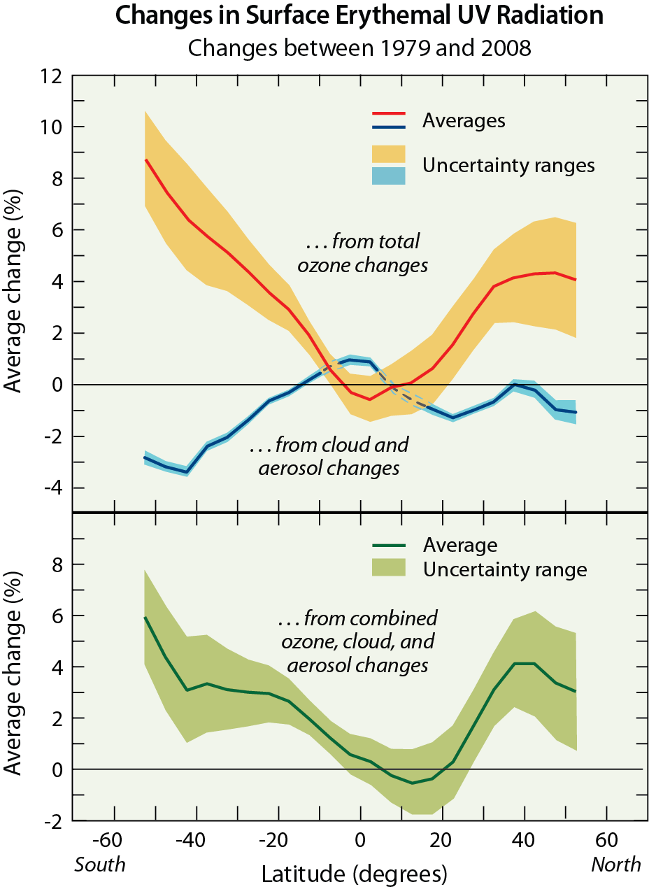
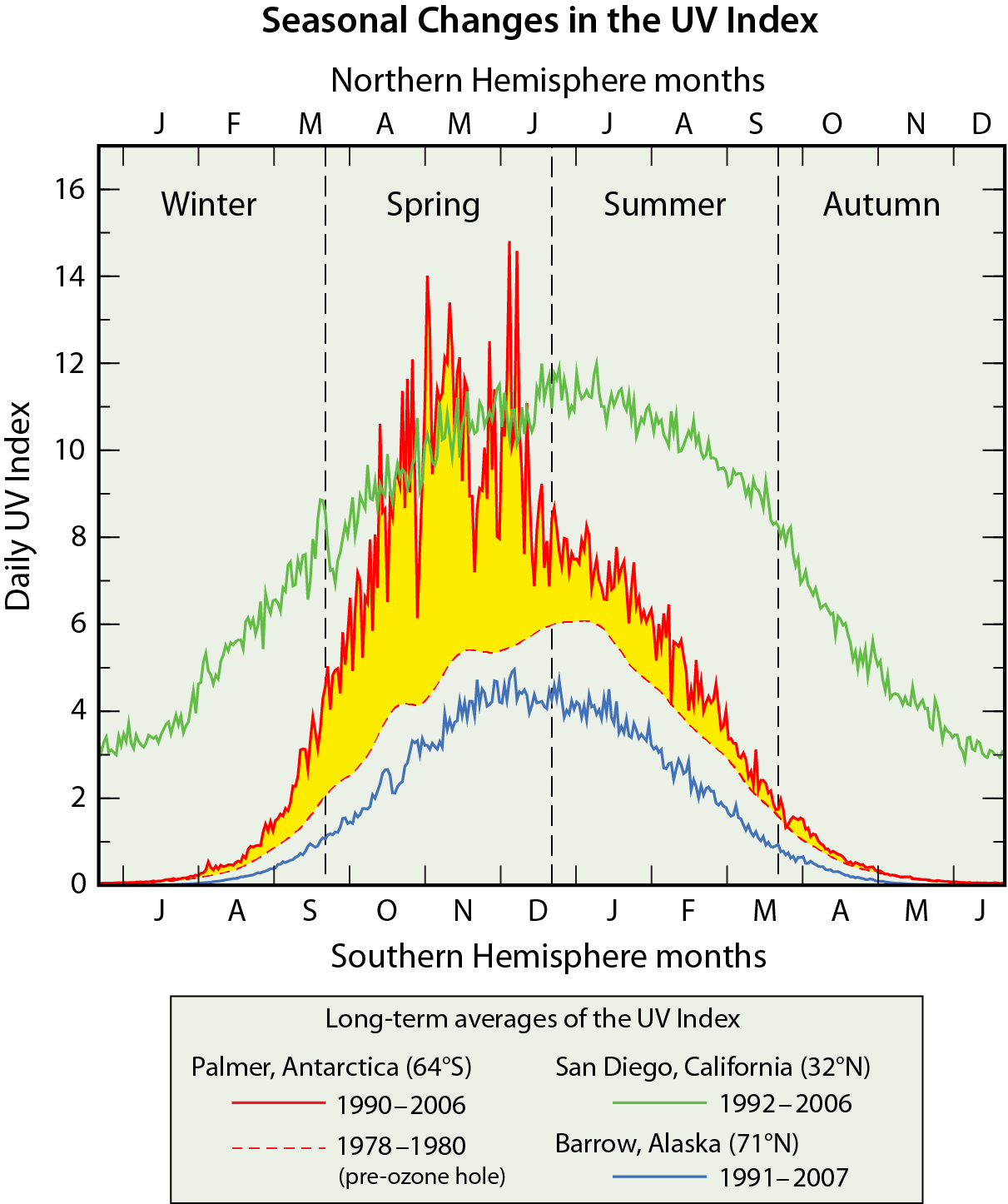
No, ozone depletion is not the principal cause of global climate change. Ozone depletion and global climate change are linked because both ozone-depleting substances and their substitutes are greenhouse gases. Ozone is also a greenhouse gas, so stratospheric ozone depletion leads to surface cooling. Conversely, increases in tropospheric ozone and other greenhouse gases lead to surface warming. The cooling from ozone depletion is small compared to the warming from the greenhouse gases responsible for observed global climate change. The Antarctic ozone hole has contributed to changes in Southern Hemisphere surface climate through effects on the atmospheric circulation.
While stratospheric ozone depletion is not the principal cause of climate change, aspects of ozone depletion and climate change are closely linked. Both processes involve gases released to the atmosphere by human activities. The links are best understood by examining the contribution to climate change of the gases involved: ozone; ozone-depleting substances (or halogen source gases) and their substitutes; and other leading greenhouse gases.
Greenhouse gases and the radiative forcing of climate. The warming of Earth by the Sun is enhanced by the presence of greenhouse gases (GHGs). The natural abundances of GHGs in Earth’s atmosphere absorb outgoing infrared radiation, trapping heat in the atmosphere and warming the surface. The most important natural GHG is water vapor. Without this natural greenhouse effect, Earth’s surface would be much colder than current conditions. Human activities have led to significant increases in the atmospheric abundances of a number of long-lived and short-lived GHGs since 1750, the start of the Industrial Era, leading to warming of Earth’s surface and associated climate changes. This group includes carbon dioxide (CO2), methane (CH4), nitrous oxide (N2O), tropospheric ozone, and halocarbons. Ozone-depleting substances (ODSs) and their substitutes make up a large fraction of the halocarbons in today’s atmosphere. Increases in the abundances of these gases from human activities cause more outgoing infrared radiation to be absorbed and reemitted back to the surface, further warming the atmosphere and surface. This change in Earth’s energy balance caused by human activities is called a radiative forcing of climate or, more simply, a climate forcing. The magnitude of this energy imbalance is usually evaluated at the top of the troposphere (tropopause) and is expressed using units of watts per square meter (W/m2). The potential for climate change rises as this radiative forcing increases.
A summary of radiative forcings of climate in 2011 resulting from the increases in the principal long-lived and short-lived GHGs from human activities since 1750 is shown in Figure Q17-1. Positive forcings generally lead to warming and negative forcings lead to cooling of Earth’s surface. Climate forcings also lead to other changes, for example reductions in glacier and sea-ice extent, variations in precipitation patterns, and more extreme weather events. International climate assessments conclude that much of the observed surface warming and changes in other climate parameters over the last several decades are due to increases in the atmospheric abundances of CO2 and other GHGs, which result from a variety of human activities.
Carbon dioxide, methane, and nitrous oxide. All three of these GHGs have both human and natural sources. The accumulation of CO2 since 1750 represents the largest climate forcing caused by human activities. Carbon dioxide concentrations continue to increase in the atmosphere primarily as the result of burning fossil fuels (coal, oil, and natural gas) for energy and transportation, as well as from cement manufacturing. The global mean atmospheric abundance of CO2 now exceeds 400 parts per million (ppm), which is more than 40% larger than the abundance of CO2 present in 1750. Carbon dioxide is considered a long-lived gas, since a significant fraction remains in the atmosphere 100– 1000 years after emission.
Methane is a short-lived climate gas (atmospheric lifetime of about 12 years). Sources related to human activities include livestock, fossil fuel extraction and use, rice agriculture, and landfills. Natural sources include wetlands, termites, and oceans. The global mean atmospheric abundance of CH4 has more than doubled since 1750.
Nitrous oxide is a long-lived climate gas (atmospheric lifetime of about 120 years). The largest source related to human activities is agriculture, especially the use of fertilizer. Microbial processes in soils that are part of natural biogeochemical cycles represent the largest natural source. In the stratosphere, nitrous oxide is the principal source of reactive nitrogen species that participate in ozone destruction cycles (see Q8). The global mean atmospheric abundance of nitrous oxide has increased by about 20% since 1750.
Halocarbons. Halocarbons in the atmosphere contribute to both ozone depletion and climate change. The halocarbons considered in Figures Q17-1 and Q17-2 are gases containing chlorine, bromine, or fluorine atoms that are either controlled under the Montreal Protocol or are GHGs that fall under the auspices of the United Nations Framework Convention on Climate Change (UNFCCC). Historically, ODSs were the only halocarbons controlled under the Montreal Protocol. In 2016, the Kigali Amendment to the Montreal Protocol established controls on the future production and consumption of certain hydrofluorocarbon (HFC) substitute gases. Perfluorocarbons (PFCs) and sulfur hexafluoride (SF6) are in the UNFCCC group of GHGs that now fall under the Paris Agreement. Perfluorocarbons are compounds that contain only carbon and fluorine atoms, such as carbon tetrafluoride (CF4) and perfluoroethane (C2F6). Technically, SF6 is not a halocarbon since it lacks carbon. However, the environmental effects of SF6 are commonly examined with those of halocarbon gases since all of these compounds contain at least one halogen atom.
In 2011, the halocarbon contribution to the radiative forcing of climate was 0.36 W/m2, which is the fourth largest GHG forcing following carbon dioxide, methane, and tropospheric ozone (see Figure Q17-1). The contributions of individual halocarbon gases are highlighted in Figure Q17-2. Within the halocarbons, CFCs contribute the largest percentage (71%) to 2011 climate forcing. The intermediate-term ODS substitutes, hydrochlorofluorocarbons (HCFCs), make the next largest contribution (14%). The long-term ODS substitutes, HFCs, contribute 5% and, finally, PFCs and SF6 contribute another 3%.
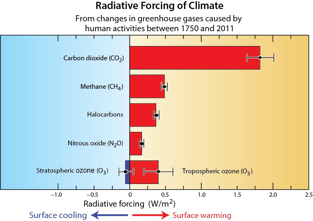
The large contribution of the CFCs has been gradually decreasing following the decline in their atmospheric abundance and is expected to further decrease (see Figure Q15-1). Based on their long lifetimes, CFCs will still make a significant contribution, and most likely the largest contribution from ODSs, to halocarbon climate forcing at the end of this century. Even with adherence to the provisions of the Kigali Amendment to the Montreal Protocol, the radiative forcing from HFCs is projected to increase for another two to three decades before starting to slowly decline (see Figure Q19-2).
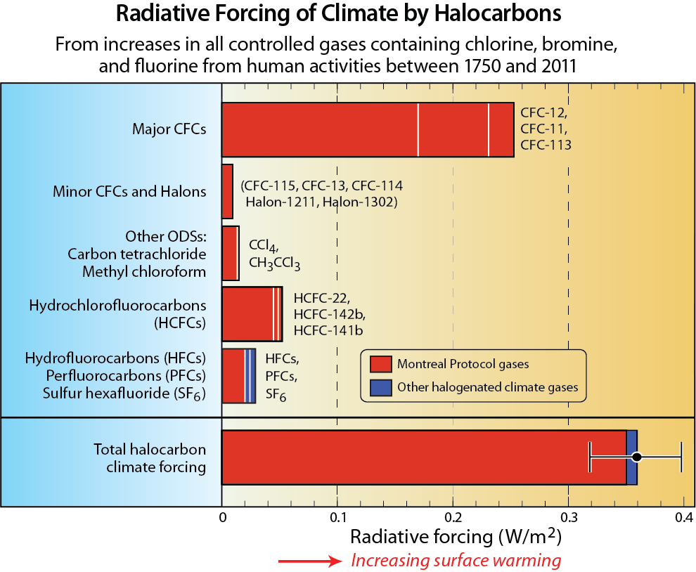
Stratospheric and tropospheric ozone. Ozone in both the stratosphere and the troposphere absorbs infrared radiation emitted from Earth’s surface, trapping heat in the atmosphere. Ozone also significantly absorbs solar ultraviolet (UV) radiation. As a result, increases or decreases in stratospheric or tropospheric ozone induce a climate forcing and, therefore, represent direct links between ozone and climate. Air pollution from a variety of human activities has led to increases in global tropospheric ozone (see Q2), causing a positive radiative forcing (warming) estimated to be +0.4 W/m2 over the 1750-2011 time period, with a range of uncertainty spanning +0.2 to +0.6 W/m2 (see Figure Q17-1). The large uncertainty in the climate forcing due to release of air pollutants reflects our limited knowledge of changes in the abundance of tropospheric ozone between 1750 and the mid-1950s as well as the difficulty in modeling the complex chemical processes that control the production of tropospheric ozone.
On the other hand, rising abundances of ODSs in the atmosphere since the middle of the 20th century have led to decreases in stratospheric ozone, most likely causing a negative radiative forcing of -0.05 W/m2 (cooling) over the 1750-2011 time period, with a range of uncertainty spanning -0.15 to +0.05 W/m2 (see Figure Q17-1). The sign of the radiative forcing due to stratospheric ozone depletion is uncertain because this quantity is the difference between two terms of comparable magnitude, each of which has an associated uncertainty. The first term represents the trapping by ozone of outgoing infrared radiation released by the surface and lower atmosphere: this is a cooling term because less ozone results in less trapping of heat. The second term represents the absorption of solar UV radiation by ozone: this is a warming term because less ozone results in greater penetration of solar UV radiation into the lower atmosphere (troposphere). The 2013 Intergovernmental Panel on Climate Change (IPCC) climate assessment concluded that stratospheric ozone depletion most likely caused a slight cooling of Earth’s surface, as shown in Figure Q17-1. This radiative forcing due to stratospheric ozone depletion will diminish in the coming decades, as ODSs are gradually removed from the atmosphere.
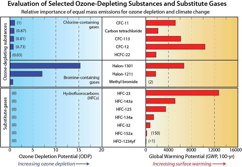
The 2013 IPCC climate assessment also evaluated the radiative effects due to changes in ozone induced solely by the release of ODSs and as well as changes in ozone caused only by air pollutants. They concluded that changes in atmospheric ozone over the 1750-2011 time period caused solely by the release of ODSs led to a cooling of -0.18 W/m2 with a range of uncertainty spanning -0.03 to -0.33 W/m2 and that changes in atmospheric ozone over the same time period caused only by release of air pollutants led to a warming of +0.50 W/m2 with a range of uncertainty spanning +0.30 to +0.70 W/m2. The radiative forcings for ozone shown in Figure Q17-1 are based on estimates of the actual changes in the abundance of stratospheric ozone and tropospheric ozone, respectively. The values given in Figure Q17-1 differ from those stated in this paragraph because some stratospheric air masses that experience loss of ozone due to human release of ODSs are transported to the troposphere, somewhat mitigating the radiative forcing of climate due to elevated amounts of tropospheric ozone caused by air pollutants. Similarly, polluted tropospheric air entering the stratosphere has led to changes in stratospheric composition that have slightly offset the decline in ozone caused solely by ozone-depleting substances.
It is clear that stratospheric ozone depletion is not a principal cause of present-day global warming. First, the climate forcing from ozone depletion is small and very likely acts to cool Earth’s surface. Second, the total radiative forcing of climate from other GHGs such as carbon dioxide, methane, halocarbons, and nitrous oxide is large and positive, leading to warming (see Figure Q17-1). The total forcing from these other GHGs is the principal cause of the observed warming of Earth’s surface.
Ozone Depletion Potentials and Global Warming Potentials. A useful way of comparing the influence of individual emissions of halocarbons on ozone depletion and climate change is to compare Ozone Depletion Potentials (ODPs) and Global Warming Potentials (GWPs). The ODP and GWP are the effectiveness of an emission of a gas in causing ozone depletion and climate forcing, respectively, relative to a reference gas (see Table Q6-1). The principal halocarbon gases are contrasted with each other in Figure Q17-3. The ODP of CFC-11 and the GWP of carbon dioxide are assigned reference values of 1. The CFCs and carbon tetrachloride all have ODPs near 1, indicating comparable effectiveness in causing ozone depletion per mass emitted. The principal halons have ODPs greater than 7, making them the most effective ozone-depleting substances per mass emitted. All HFCs have ODPs of zero since they contain no chlorine and bromine, and therefore do not directly cause ozone depletion (see Q6).
All halocarbons have non-zero GWPs and, therefore, contribute to the radiative forcing of climate. The GWP does not correspond strongly with the ODP of a gas because these quantities depend on different chemical and physical properties of the molecule. For example, while HFC-143a does not destroy ozone (ODP equals zero), each gram emitted is about 5000 times more effective than a gram of carbon dioxide in causing climate forcing. When HFCs are released to the atmosphere, their contribution to climate forcing depends on their GWPs, which vary over a wide range (less than 1 to 13,000).
Montreal Protocol regulations have led to reductions in CFC emissions and increases in HCFC emissions (see Q15). As a result of these actions, the total radiative forcing from ODSs stopped increasing and is now slowly decreasing (see Q18). Overall halocarbon radiative forcing, however, is slowly increasing because of growing contributions from non-ODS gases (HFCs, PFCs, and SF6). The growth in the HFC contribution will be limited by the provisions of the 2016 Kigali Amendment (see Q19). It is important to note that despite having a GWP that is small in comparison to many other halocarbons and other greenhouse gases, carbon dioxide is the most important greenhouse gas produced by human activities because its emissions are large, its atmospheric lifetime is long, and its atmospheric abundance is far greater than those of all other greenhouse gases associated with human activities.
The Antarctic ozone hole and Southern Hemisphere climate. While stratospheric ozone depletion is not the principal cause of global climate change, the reoccurring Antarctic ozone hole has contributed to observed changes in climate parameters in the atmosphere and oceans of the Southern Hemisphere. These research findings are explained in more detail in the box below.
Yes. Many ozone-depleting substances (ODSs) are also potent greenhouse gases that contribute to climate forcing when they accumulate in the atmosphere. Montreal Protocol controls have led to a substantial reduction in the emissions of ODSs over the last two decades. These reductions, while protecting the ozone layer, have the additional benefit of reducing the human contribution to climate change. Without Montreal Protocol controls, the climate forcing due to ODSs could now be nearly two and a half times the present value.
The success of the Montreal Protocol in controlling the production and consumption of ozone-depleting substances (ODSs) has protected the ozone layer (see Q14). The resulting reductions in atmospheric abundances of ODSs also decreased the human influence on climate because all ODSs are greenhouse gases (see Q17). By protecting both ozone and climate, the Montreal Protocol has provided a dual benefit to society and Earth’s ecosystems. As shown in Figure Q18-1 and described below, the dual benefit of the Montreal Protocol is highlighted by considering a long-term baseline and a world-avoided scenario of ODS emissions that use Ozone Depletion Potentials (ODPs), Global Warming Potentials (GWPs), equivalent effective stratospheric chlorine (EESC), and the radiative forcing of climate.
Baseline ODS scenario. The baseline scenario refers to actual past ODS emissions of the principal halogen source gases and projected emissions for the years 2017 to 2020. The baseline scenario is labeled “From observed ODS abundances” in Figure Q18-1 since, for 1960–2016, the emissions are based upon analysis of observed abundances of the principal ODS gases at Earth’s surface (see Figure Q15-1). This scenario also includes emissions of the naturally occurring halogen source gases methyl chloride (CH3Cl) and methyl bromide (CH3Br). For this scenario the peak emission of ODSs occurs in the late 1980s (see Figure Q0-1).
For all of the emission scenarios shown in Figure Q18-1, the annual emissions of each gas are added together after being weighted (multiplied) by their corresponding Ozone Depletion Potential (ODP) (upper left) or Global Warming Potential (GWP) (upper right) (see Q17 and Table Q6-1). In the ODP-weighted scenario, the sum of emissions is expressed as CFC-11-equivalent emissions because CFC-11 is the reference gas, with an assigned ODP value of 1. For example, in the sum, 1 kg of halon-1211 emissions is added as 6.9 kg of CFC-11-equivalent emissions because the ODP of halon-1211 is 6.9. Similarly, the GWP-weighted sum is expressed as CO2-equivalent emissions because CO2 is the reference gas, with an assigned GWP of 1. For example, in the sum, 1 kg of carbon tetrachloride emissions is added as 2110 kg of CO2-equivalent emissions because the GWP of carbon tetrachloride is 2110.
World-avoided ODS scenario. The baseline scenario of ODS emissions can be contrasted with a scenario of ODS emissions that the world has avoided by successfully implementing the Montreal Protocol (see Figure Q18-1). The world-avoided scenario is derived by assuming that emissions of ODSs in the baseline scenario increase beyond 1987 values at a 3% annual growth rate. This growth rate is consistent with the strong market for ODSs in the late 1980s that included a wide variety of current and potential applications and had the potential for substantial growth in developing countries.
CO2 emission scenario. Long-term emissions of CO2 are also shown in the upper right panel of Figure 18-1. Atmospheric CO2 is the principal greenhouse gas emitted by human activities. The CO2 emission curve represents global emissions from the sum of each nation’s reported emissions from the combustion of coal, oil, natural gas, the fuels used by the world’s ships and airplanes, cement manufacturing, and the release of CO2 due to global deforestation.
ODP-weighted emissions. The ODP-weighted emission scenario based upon observed ODS abundances is one measure of how the overall threat to stratospheric ozone from ODSs has changed over time (see Figure Q18-1, upper left panel). When ODP-weighted emissions increase in a given year, more ozone will be destroyed in future years relative to the amount of ozone depletion caused by the emissions in the prior year. Conversely, when emissions decline, less ozone will be destroyed in future years. Annual ODP-weighted emissions increased substantially between 1960 and 1987, the year the Montreal Protocol was signed (see Figure Q0-1). After 1987, annual ODP-weighted emissions began a long and steady decline to present-day values. The decline in emissions is expected to continue, causing the atmospheric abundances of all individual ODSs to eventually decrease (see Figure Q15-1). The reductions in ODP-weighted emissions following the peak value in 1987 represent lower limits of the annual emissions avoided by the Montreal Protocol, which are a measure of its increasing success over time in protecting the ozone layer.
The upper limits of annual reductions in ODP-weighted emissions are derived from the world-avoided scenario. The difference between the world-avoided emission scenario and the baseline scenario (blue shaded region in Figure Q18-1, upper left panel) provides a reasonable upper limit to the ODP-weighted emissions that have been avoided by the Montreal Protocol since 1987. The avoided emissions are a measure of the ozone layer protection afforded by the Protocol. If the emissions of ODSs had followed the world avoided scenario, annual ODP-weighted emissions in 2018 would be more than 10 times the current value.
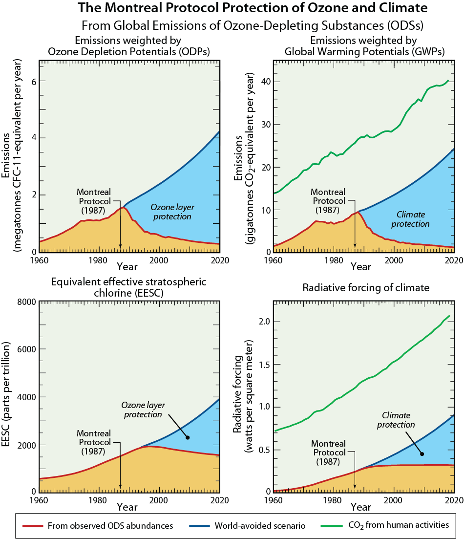
(A megatonne = 1 million (106) metric tons = 1 billion (109) kilograms. A gigatonne = 1 billion (109) metric tons = 1 trillion (1012) kilograms. The CFC-11-equivalent emission unit means release of an ODS would result in the same amount of ozone depletion as release of the same mass of CFC-11; the CO2-equivalent emission unit means release of a GHG would result in the same amount of RF of climate as release of the same mass of CO2, over a 100-year time interval. Emissions of CO2 used in this figure are from the Global Carbon Project.)
GWP-weighted emissions. The GWP-weighted emission scenario based upon observed ODS abundances is a measure of how the overall threat to Earth’s climate from ODSs has changed over time (see Figure Q18-1, upper right panel). As GWP-weighted emissions rise, the radiative forcing of climate in the future due to the accumulation of ODSs in the atmosphere also increases. The long-term changes in the GWP-weighted scenario are very similar to those in the ODP-weighted scenario. Both show an increase before 1987 and a decrease afterwards. The similarity follows from the predominant role that CFC-11 and CFC-12 emissions play in ozone depletion and climate forcing from ODSs. The reductions in GWP-weighted emissions since the 1987 peak represent lower limits of the annual emissions avoided by the Montreal Protocol, which are a measure of its climate protection from human activities. The difference between the world-avoided emission scenario and the baseline scenario (blue shaded region in Figure Q18-1, upper right panel) provide an estimated upper limits to the GWP-weighted emissions avoided by the Montreal Protocol since 1987. If the emissions of ODSs had followed the world avoided scenario, annual GWP-weighted emissions in 2018 would be more than 10 times the current value.
Annual GWP-weighted emissions of ODSs were a large percentage (about 20–40%) of global emissions of CO2 between 1960 and 1987. Thereafter, this percentage has steadily decreased and was 2–3% of global CO2 emissions in 2018. This past trend stands in sharp contrast to the world-avoided scenario, in which emissions of ODSs are more than 50% of CO2 emissions in 2018. Another way to understand the climate benefit of the Montreal Protocol is to compare the height of the blue shaded region in 2018 to the rise in the emissions of CO2 since 1987, as shown in Figure Q18-1 (upper right panel). These two quantities are nearly equal in magnitude, demonstrating that since 1987 the Montreal Protocol has avoided an increase in GWP-weighted emissions of ODSs that nearly equals the increase in global emissions of CO2 over this same period of time.
EESC scenarios. The EESC scenarios in Figure Q18-1 (lower left panel) provide a measure of the year-to-year potential of the atmospheric abundances of ODSs to destroy stratospheric ozone. Two scenarios are shown: the baseline that is based on observed abundances of ODSs (with a projection to 2020) and the world-avoided scenario described above. The derivation of EESC from ODS atmospheric abundances is discussed in Q15 and the same EESC baseline scenario is shown in Figures Q13-1, Q14-1 (red curve), and Q15-1 for different time intervals. When ODS-weighted emissions declined after 1987, EESC did not decrease in a proportional manner because of the long atmospheric lifetimes of the principal ODSs (see Table Q6-1). As shown in Figure Q18-1, EESC reached its peak value nearly a decade after the peak in ODP-weighted emissions, and by 2018 the decrease in EESC from its peak value was only about 18%, compared to the 80% decrease in ODP-weighted emissions achieved by 2018. Conversely, had the emissions of ODSs followed the world-avoided scenario, EESC would be more than twice the value in today’s stratosphere. In this case, computer simulations indicate that in the year 2020, global total ozone would have been about 17% lower than the 1964–1980 average. Even larger depletions would have occurred in subsequent years. The Montreal Protocol and its Amendments and Adjustments have provided vitally important protection to the global ozone layer and climate.
Radiative forcing scenarios. The scenarios for radiative forcing in Figure 18-1 (lower right panel) provide a measure of the year-to-year contribution to climate change from the atmospheric abundances of ODSs. The radiative forcing of an ODS is equal to the net increase in its atmospheric abundance since 1750 multiplied by its radiative efficiency. Increases in abundance up to the present are derived from atmospheric observations. The radiative forcing due to ODSs increases smoothly from 1960 onward, peaks in 2010, and decreases very gradually in subsequent years. The response of radiative forcing to ODS emission reductions is a slow decline attributable to the high abundances of the two principal contributing gases, CFC-11 and CFC-12, and their long atmospheric lifetimes (50–100 years).
Increasing the benefits of the Montreal Protocol. The benefits of the Montreal Protocol for protection of the ozone layer and climate could be further increased by the expanded capture and destruction of halons, chlorofluorocarbons (CFCs), and hydrochlorofluorocarbons (HCFCs) in banks, by avoiding emissions in continued use of ODSs, and by eliminating future emissions of halogen source gases not controlled by the Montreal Protocol, such as dichloromethane (CH2Cl2). Banks are largely associated with ODSs contained in refrigeration, air conditioning, and fire protection equipment, and stockpiles for servicing long-term applications. Atmospheric release of ODSs from existing banks is projected to contribute more to ozone depletion in the coming decades than the limited production and consumption of ODSs (HCFCs and CH3Br) allowed by the Montreal Protocol after 2020. If all available options were implemented to avoid future atmospheric release of ODSs starting in 2020, the return of EESC to 1980 values would be advanced by about a decade for both the midlatitude (see Figure Q14-1) and polar stratosphere.
Notably, the annual decline in the atmospheric abundance of CFC-11 has slowed measurably during recent years compared to the expected decline, due to emissions from unreported production (see Q15). If these emissions of CFC-11 are assumed to continue in the coming decades at the value derived for the 2002-2016 period, the return of EESC to the 1980 value is delayed by about seven years for the midlatitude stratosphere relative to the projections for EESC shown in Figures Q14-1 and Q15-1. Similarly, the delay is about 20 years for the polar stratosphere.
At the 28th Meeting of the Parties to the Montreal Protocol held in Kigali, Rwanda, in October 2016, the Montreal Protocol was amended to control the production and consumption of hydrofluorocarbons (HFCs). The Montreal Protocol phaseout of chlorofluorocarbons (CFCs) led to the temporary use of hydrochlorofluorocarbons (HCFCs). The subsequent phaseout of HCFCs led to expanded long-term use of HFCs, because HFCs pose no threat to the ozone layer. However, HFCs are greenhouse gases and therefore contribute to climate change. Limiting the production and consumption of those HFCs with high global warming potentials is projected to avoid 0.2 to 0.4°C of global warming over this century. The Kigali Amendment marks the first time the Montreal Protocol has adopted regulations solely for the protection of climate.
The control of ozone-depleting substances (ODSs) by the Montreal Protocol provides the dual benefit of protecting Earth’s ozone layer and global climate (see Q18). The widespread global use of hydrofluorocarbons (HFCs) and their projected future growth in the coming decades has been recognized by the Montreal Protocol as a potentially significant contribution to climate change from human activities. In response, the Kigali Amendment was adopted to control production and consumption of HFCs with high Global Warming Potentials (GWPs) (see Q17). Full compliance with the provisions of the Kigali Amendment to the Montreal Protocol will significantly enhance the climate-protection benefit of this international agreement.
Hydrofluorocarbons (HFCs). HFCs are replacement compounds for ODSs that were chosen because they contain no chlorine or bromine that cause ozone depletion. HFCs are widely used in the refrigeration and air-conditioning sectors, as foam-blowing agents and spray can propellants, as well as feedstocks for the production of other chemicals. These uses are growing as the global phaseout of hydrochlorofluorocarbons (HCFCs), the early replacement compounds, nears completion. The GWPs of HFCs vary over a wide range due to differences in their physical and radiative properties (see Table Q6-1 and Figure Q17-3). For example, the GWP of HFC-134a (primarily used in air conditioning and refrigeration) is 1360, which means that after release to the atmosphere, each kilogram of HFC-134a is 1360 times more effective than a kilogram of CO2 in increasing climate forcing over a century-long time period. In contrast, the GWP of HFO-1234yf, a substitute for HFC-134a, is less than 1.
HFC-23. HFC-23 is considered separately in the Kigali Amendment because this gas is primarily formed as an unwanted byproduct in the production of HCFC-22. The global warming potential of HFC-23 is quite large (12,690), in part due to its long atmospheric lifetime of 228 years. Although many methods exist to chemically destroy HFC-23 at production facilities, this compound continues to be released to the atmosphere. For example, the atmospheric abundance of HFC-23 increased by 28% between 2009 and 2016. In 2016, the climate forcing of HFC-23 was 0.005 W/m2, which is approximately 17% of the total forcing from all HFCs. The Kigali Amendment phases down, in conjunction with the other HFCs, unwanted by-production of HFC-23, but provides no specific control measures for emissions of HFC-23. Instead, the Amendment encourages nations to destroy HFC-23 to the extent practicable in order to avoid future emissions and the associated increased climate forcing.
Climate implications of HFC use. The total global emission of HFCs expressed in terms of CO2-equivalent emissions has grown steadily since 2000, approaching 1 gigatonne CO2-equivalent per year in 2016 (see Figure Q19-1). The primary emissions of HFCs are of HFC-134a as well as HFC-143a and HFC-125, which are widely used in blended refrigerants such as R404A (52% HFC-143a, 44% HFC-125, and 4% HFC-134a) and R410A (50% HFC-32, 50% HFC-134a). Recent growth in the emissions of HFCs is due in part to replacing HCFCs that are being phased out under the Montreal Protocol. Currently, the atmospheric abundances of HFCs contribute about 5% of climate forcing from all halocarbon compounds (see Figure Q17-2) and less than 1% of the total climate forcing from all other greenhouse gases (see Figure Q17-1). Projections based on current production and consumption patterns and future economic growth indicate that, without the Kigali Amendment, HFC emissions could reach around 5 gigatonnes CO2-equivalent per year by 2050 and nearly double that value by 2100. This projected emission value for 2050 is about one half of the peak in CO2-equivalent emissions of ODSs in 1987 (see Figure Q18-1). Thus, in the absence of the Kigali Amendment, the projected growth in HFC emissions in the coming decades would offset a significant amount of the climate protection gained from reductions in ODS emissions under the Montreal Protocol.
Kigali Amendment. The future of HFC emissions was changed by the Montreal Protocol with the adoption of the Kigali Amendment in 2016. The amendment requires a phasedown of the global production and consumption of high-GWP HFCs by more than 80 percent (in CO2-equivalent) from the baseline level over the next 30 years. The phasedown schedule accommodates the concerns and interests of developed and developing countries, including those with high ambient temperatures. The Kigali Amendment entered into force on 1 January 2019. Figure Q19-1 shows how the Amendment dramatically reduces projected emissions of HFCs in the coming decades. The emissions of HFCs that are avoided by 2100 total about 420 gigatonnes CO2-equivalent, which is more than 10 years of present-day annual emissions of CO2 due to human activities.
Expanding climate protection. The Kigali Amendment substantially expands the protection of climate afforded by the Montreal Protocol (see Q18). With full implementation of the Amendment, annual global emissions of HFCs reach their peak value before 2040 (see Figure Q19-1). Without the Amendment, yearly emissions increase until market saturation is reached in the second half of the century, at a value of about 10 gigatonnes CO2-equivalent per year, nearly five times more than the emission peak under the Amendment. Furthermore, as shown in Figure Q19-2, the long-term radiative forcing of climate, which is proportional to atmospheric abundances, is substantially reduced. Without the Amendment, projected climate forcing from HFCs increases throughout this century, reaching a value of about 0.6 W/m2 in 2100. In this scenario, climate forcing due to HFCs by the end of the century exceeds that of nitrous oxide and rivals that of methane. With the Amendment, the radiative forcing of climate by HFCs reaches a peak value before 2050 and gradually decreases to about 0.09 W/m2 in 2100. The ranges of climate forcing values for methane and nitrous oxide in 2100 as shown in Figure Q19-2 far exceed the 0.09 W/m2 forcing due to HFCs under the Kigali Amendment.

(A gigatonne = 1 billion (109) metric tons = 1 trillion (1012) kilograms. The CO2-equivalent emission unit means release of a GHG would result in the same amount of radiative forcing of climate as release of the same mass of CO2, over a 100-year time interval.)
The benefit of reducing climate forcing over many decades under the Amendment can be expressed as an avoided increase in globally averaged surface temperature. The increase in temperature by the year 2100 due to future atmospheric growth of HFCs without the Kigali Amendment and national regulations is projected to be between 0.3 and 0.5°C (see Figure Q19-2). In contrast, the temperature increase is projected to be about 0.06°C with full implementation of the Amendment, which is significantly less, for example, than the warming expected from projected abundances of methane and nitrous oxide in 2100. Currently, global warming due to all emissions from human activities is about 1°C since 1750, the start of the Industrial Era. The goal of the United Nations Framework Convention on Climate Change Paris Agreement is to limit global warming to well below 2.0°C since the start of the Industrial Era and to pursue efforts to limit global warming to 1.5°C. The temperature increase of 0.2 to 0.4°C avoided by the Kigali Amendment contributes substantially to the achievability of this goal.
Low-GWP substances. The Kigali Amendment encourages the use of low-GWP substances or other alternatives to replace high-GWP HFCs in the coming decades (see Table Q6-1 and Figure Q17-3). The HFC replacement compounds include a subset of HFCs known as hydrofluoroolefins (HFOs), which, like HFCs, are composed only of hydrogen, fluorine and carbon atoms. The chemical structure of HFOs includes a double carbon bond, causing these compounds to be more reactive in the lower atmosphere (troposphere) than other HFCs. Consequently, HFOs have very short atmospheric lifetimes. One such compound, HFO-1234yf, has a lifetime of only 12 days, in contrast to HFC-23, HFC-143a, and HFC-134a with lifetimes of 228, 51, and 14 years, respectively (see Table Q6-1). The short atmospheric lifetimes of HFOs lead to very low GWPs. As a result, the emission of an HFO results in substantially lower climate forcing than the forcing caused by emission of the same mass of high-GWP HFCs (see Figure Q19-1).
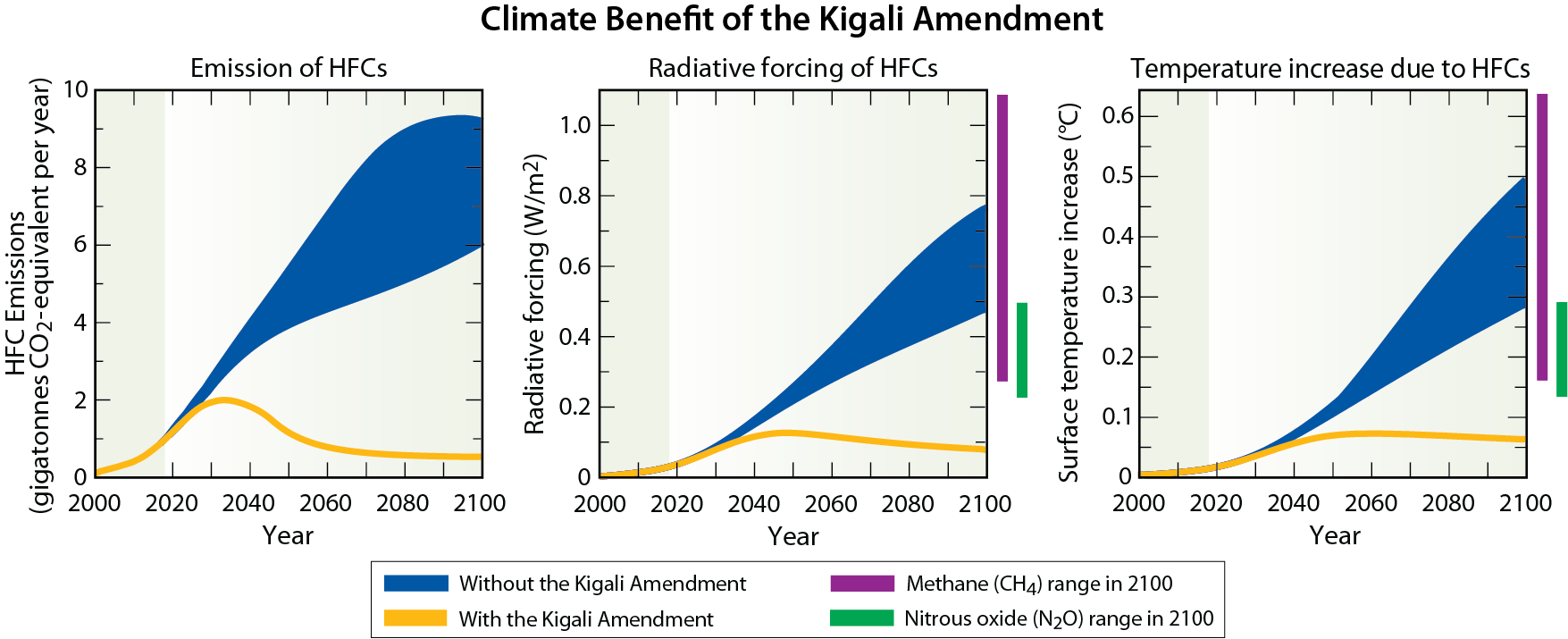
(A gigatonne = 1 billion (109) metric tons = 1 trillion (1012) kilograms. The CO2-equivalent emission unit means release of a GHG would result in the same amount of radiative forcing of climate as release of the same mass of CO2, over a 100-year time interval. The end of century values for CH4 and N2O are based upon the Representative Concentration Pathway (RCP) 2.6 (lower limit) and 8.5 (upper limit) scenarios.)
The projections of emissions under the Kigali Amendment include a group of compounds labeled Low-GWP Alternatives in Figure Q19-1. These compounds are expected to cover the application demand from sectors in which the use of high-GWP HFCs is phased down. Even with the emissions of a large mass of these low-GWP alternatives in future projections, the contribution to climate change remains low in comparison to the contributions from future emissions of high-GWP HFCs that would occur without the Kigali Amendment.
The Future. The phasedown of HFCs under the Kigali Amendment sets a path in which HFCs play a very limited role in future climate forcing. Achieving the maximum climate protection from the implementation of the Amendment requires that compounds replacing high-GWP HFCs have smaller or negligible GWPs. Technological developments related to new low-GWP substances and improved refrigeration and air conditioning equipment will help maximize the protection of climate. The release of greenhouse gases in generating electricity for powering refrigeration and air conditioning equipment contributes to the indirect climate forcing from this sector. Improvements in the energy efficiency of equipment in this sector during the transition to low-GWP alternative refrigerants could potentially double the direct climate benefits of the Amendment. The combination of low-GWP replacement compounds, energy efficiency improvements, and the growth in renewable energy sources has great potential to minimize the direct and indirect contributions to climate forcing from global refrigeration and air conditioning applications.
Stratospheric ozone in the future
Substantial recovery of the ozone layer from the effects of ozone-depleting substances (ODSs) is expected around the middle of the 21st century, assuming global compliance with the Montreal Protocol. Recovery will occur as ODSs and reactive halogen gas abundances in the stratosphere decrease in the coming decades. In addition to responding to ODSs, ozone abundances are increasingly being influenced by climate change. The impacts of future climate change on the ozone layer will vary between the tropics, midlatitudes, and polar regions, and strongly depend on future emissions of carbon dioxide (CO2 ), methane (CH4), and nitrous oxide (N2O). During the long recovery period, large volcanic eruptions could temporarily reduce global ozone amounts for several years.
Substantial recovery from the depletion of global and polar ozone caused by ozone-depleting substances (ODSs) is expected in the middle of this century. The recovery follows from the success of the Montreal Protocol in reducing the global production and consumption of ODSs. Currently, the atmospheric abundances of most major ODSs and the associated annual values of equivalent effective stratospheric chlorine (EESC) are in decline (see Q15). In contrast to the diminishing role of ODSs, changes in climate are expected to have an increasing influence on future levels of total ozone. Climate change is driven by the projected growth in the abundance of greenhouse gases (GHGs), primarily carbon dioxide (CO2 ), methane (CH4 ), and nitrous oxide (N2O). Rising abundances of GHGs will lead to changes in temperature, chemistry, and the circulation of the stratosphere, all of which affect ozone. Chemistry-climate models can be used to project how ozone is expected to respond to changes in ODSs and climate in particular geographical regions during the recovery period. Global events, such as major volcanic eruptions or actions to mitigate global warming by geoengineering, may also influence future ozone levels.
Using chemistry-climate models. Projections of total ozone presented here are based on the results from a group of chemistry-climate models that account for the influences of changes in ODSs and GHGs. These models show how changes in ozone are expected to vary across geographic regions by evaluating the complex interactions of the processes that control ozone and climate involving radiation, chemistry, and transport. Model inputs include historical and projected concentrations of ODSs, CO2, CH4, N2O, air pollutant gases, as well as solar output. The results from chemistry-climate model simulations are used to identify particular processes that are important for future abundances of ozone. For example, model projections for the coming decades show a strengthening in the atmospheric circulation that brings air from the troposphere into the stratosphere in the tropics, moves air poleward into both hemispheres, and then returns air to the troposphere at middle to high latitudes. These circulation changes will significantly alter the global distribution of ozone and the atmospheric lifetimes of ODSs and other long-lived gases. Also, while Earth’s surface is expected to continue to warm in response to positive radiative forcing (RF) of climate from GHGs (see Q17), the stratosphere is expected to continue to cool. A colder upper stratosphere leads to increases in ozone because lower temperatures slow down the gas-phase reactions responsible for ozone loss (see box in Q12). Finally, methane and nitrous oxide are both involved in the chemistry that determines future levels of stratospheric ozone.
Simulating recent ozone changes. Comparisons of model results with observations help confirm the causes of ozone depletion and increase confidence in model projections of future ozone amounts. Two important measures are the globally averaged total column ozone (see Q3) as well as total ozone in the Antarctic during October (the month of peak ozone depletion). These are compared to a group of chemistry-climate model simulations in Figure Q20-1. Both measures of ozone show substantial depletion since 1980. The average model values of ozone follow the observed general decline in both of these measures, suggesting that the main processes involved in ozone depletion are reasonably well represented by these models. There are significant year-to-year variations in global and Antarctic ozone that are not captured by these simulations. The differences between the observed and modeled values of ozone are due to factors such as interannual meteorological variability and volcanic eruptions that are not well represented in these simulations. Over the past few years, observed global ozone has been about 2.2% lower than the 1964-1980 average and has exhibited no statistically significant trend (see Figure Q12-1). Antarctic ozone during October has exhibited considerable variability with no strong trend over the past 20 years (see Figure Q20-1). However, there are emerging indications that the ozone hole has diminished in size and depth (maximum amount of ozone depletion) since 2000, particularly during early spring (see Figure Q10-2 and box in Q12).
Equivalent effective stratospheric chlorine (EESC) projections. Equivalent effective stratospheric chlorine (EESC) represents how the potential for reactive chlorine and bromine gases to destroy ozone varies over time (see Q15). Output from chemistry-climate models is used to compute EESC as a function of altitude, latitude, longitude, and time. These calculations are based on the history and projections of ODS surface abundances and the chemical and transport processes that control (1) the conversion of ODSs to reactive halogen gases, (2) the distribution of reactive halogen gases in the global stratosphere, and (3) their ultimate removal from the stratosphere. Long-term changes in EESC for five geographic regions as well as the global average are shown in Figure Q20-2 as the differences relative to the amount present in 1960. For all regions, values of EESC increase smoothly with time starting in 1960, reach a peak near the end of the past century, and decrease gradually until the end of this century. Global and regional values of EESC at the end of this century are very near their 1960 values, indicating that ODSs are largely removed from the stratosphere by that time.
Peak values of EESC, which occur around the year 2000, are highest in the polar regions and lowest in the tropics. In the tropics, stratospheric air has only recently been transported from the troposphere, with the result that only a small fraction of ODSs has undergone conversion to reactive halogen gases (see Q7 and Q12). In polar regions, this fraction is much larger because more conversion can occur over the several years it takes stratospheric air to journey from entry points in the tropics to the stratosphere in both polar regions.
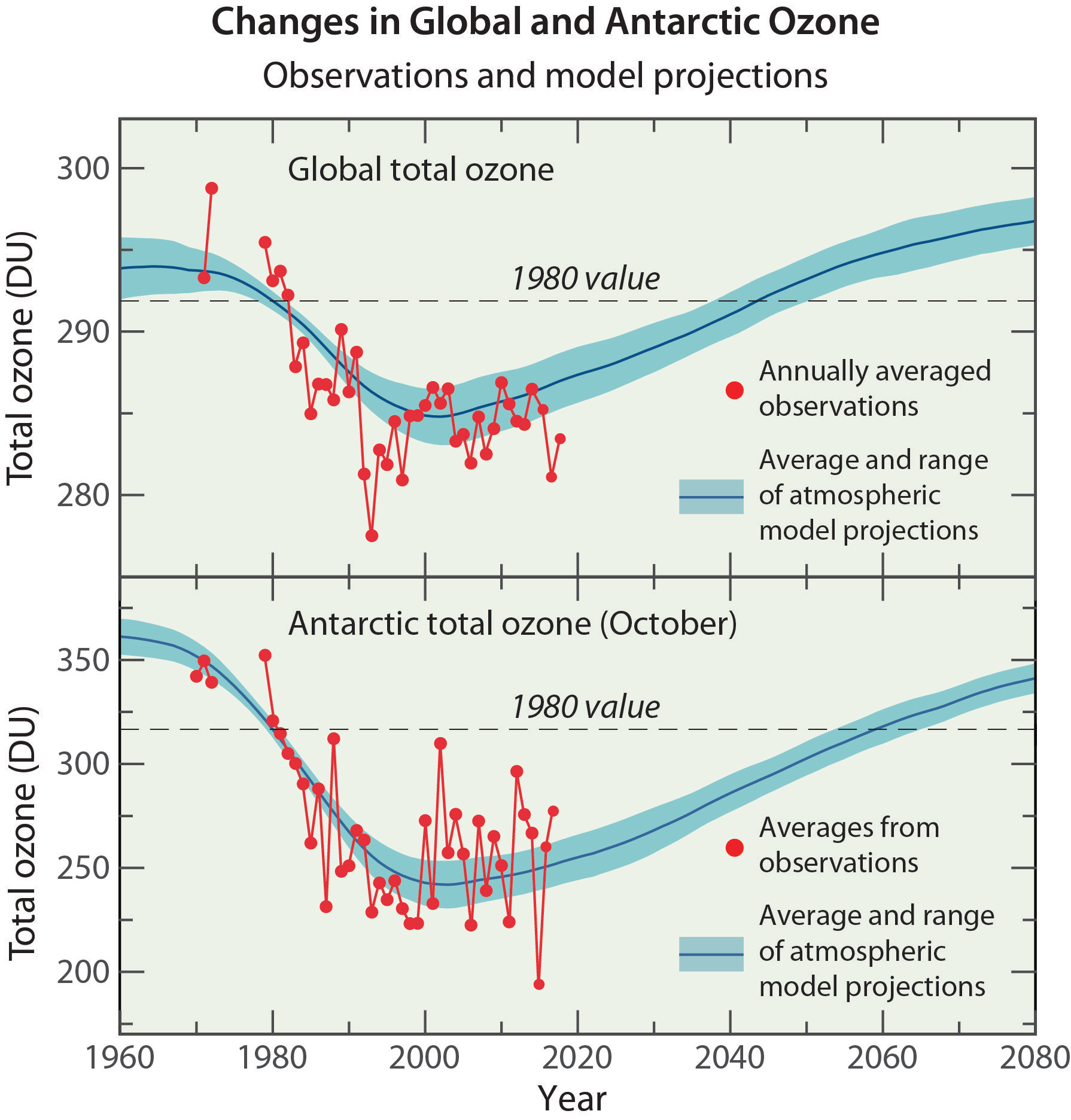
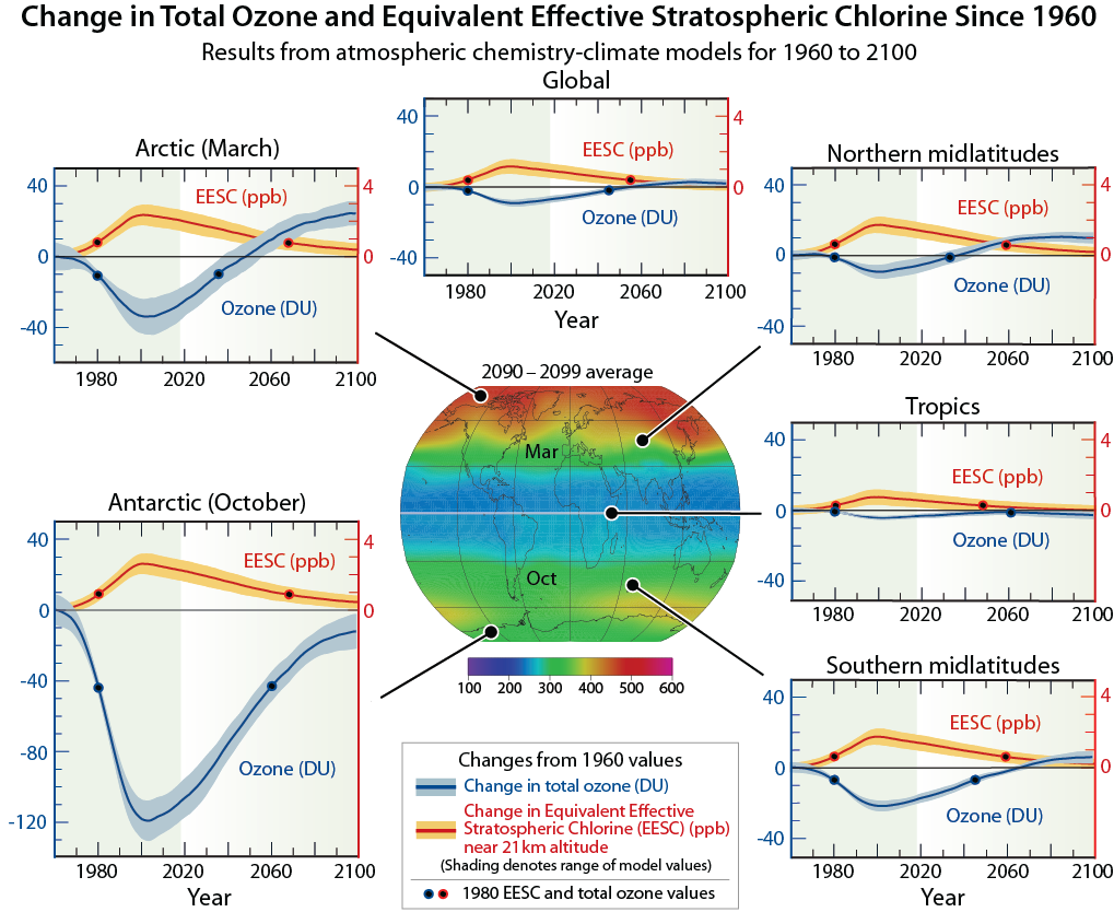
(The CCM projections utilize abundances of GHGs from the RCP 6.0 scenario and ODSs from the baseline (A1) scenario of the 2010 Scientific Assessment of Ozone Depletion report. The quantity termed EESC in this figure is sometimes referred to as Equivalent Stratospheric Chlorine (ESC) when derived from the output of chemistry-climate models.)
Long-term total ozone projections. Total ozone changes derived from chemistry-climate models, referenced to 1960 values, are shown for 1960 to 2100 in Figure Q20-2. The range of values from the group of models is included in the figure as one measure of the uncertainty in the model projections. These simulations utilize abundances of CO2, CH4, and N2O from a particular projection developed for climate models termed Representative Concentration Pathway 6.0 (RCP6.0), coupled with the projected abundances of ODSs given in the 2010 Scientific Assessment of Ozone Depletion report (see caption). Total ozone changes in the various regions are described as follows:
Antarctic. Total ozone changes are largest in the Antarctic region in springtime (October). Chemistry-climate models show that ODSs are the predominant factor in Antarctic ozone depletion in the past and in the coming decades. Changes in climate parameters have a smaller role. As a reult, changes in total ozone mostly mirror changes in EESC: as EESC increases, ozone proportionately decreases; as EESC decreases, ozone proportionately increases. Meteorological variability in the Antarctic in late winter/early spring when ozone depletion occurs causes a large range in the model projections. Antarctic total ozone is projected to return to 1980 levels after midcentury, which is later than found for most other regions.
Arctic. Total ozone changes in the Arctic region in spring-time (March) are considerably smaller than in the Antarctic. In contrast to the Antarctic, ozone changes do not closely mirror changes in EESC. After midcentury, Arctic total ozone increases to values above those that would be expected from EESC reductions alone because of the strengthening of atmospheric circulation and enhanced stratospheric cooling associated with increases in GHGs such as CO2. By 2100 Arctic total ozone is projected to be well above both the 1960 and 1980 values. The large range in projections compared to other nonpolar regions is due to greater meteorological variability, as noted for the Antarctic. Arctic total ozone is projected to return to the 1980 level in the mid-2030s, about three decades before EESC returns to its 1980 level.
Northern and southern midlatitudes. The annual averages of total ozone changes in midlatitudes are much smaller than the springtime losses in polar regions. In the northern midlatitudes, the models predict a return of total ozone to the 1960 value in the early 2030s, whereas EESC requires the full century to return close to the 1960 value. In the southern midlatitudes, total ozone returns to the 1960 level by mid-century, somewhat later than found for the Northern Hemisphere. The maximum ozone depletion near the year 2000 is much larger for the Southern Hemisphere, and total ozone more closely follows EESC. This behavior reflects the influence of the Antarctic ozone hole on the southern mid-latitudes from the transport of ozone-depleted air following the breakup of the polar vortex in late spring (see Q10). The more rapid return of total ozone to 1960 values for both regions, compared to the return of EESC, reflects the influence of climate-induced changes in stratospheric circulation and upper stratospheric temperatures. After returning to the 1960 value, total ozone continues to increase in both hemispheres and significantly exceeds that value by 2100.
Tropics. Total ozone changes in the tropics are smaller than in any other region. Ozone is less sensitive to ODSs in the tropical stratosphere because of the dominant roles of production and transport in controlling ozone and the low amounts of EESC available in this region. In contrast to other regions, chemistry-climate models project total ozone to remain below the 1960 value throughout this century. Total ozone gradually returns to the 1980 level around 2060, and then decreases gradually until the end of the century. The decline of tropical ozone during the latter part of the century is primarily due to a strengthening of the stratospheric circulation, which leads to enhanced transport of ozone out of the tropics and into midlatitudes. This circulation change also influences the Arctic and midlatitude regions, as noted above.
The globe. The annual average of global (60°S to 60°N) total ozone is projected to return to the 1960 level around 2060, while EESC returns to its 1960 value near the end of the century. Ozone returns to the 1980 value near 2047, about a decade prior to the return of EESC to its 1980 level. By the end of the century the abundance of global total ozone is projected to be 3 DU larger than the 1960 level, a 1% increase. Chemistry-climate model analysis suggests the early return of total ozone relative to EESC, as well as the end of century rise, are primarily a result of upper stratospheric cooling.
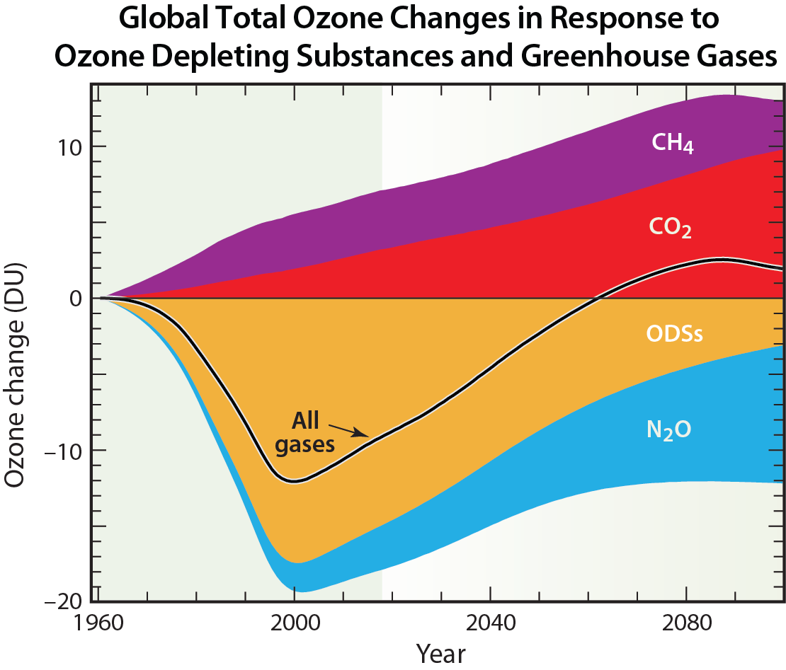
(These projections utilize abundances for CO2, CH4, N2O from the RCP 6.0 scenario and ODSs from the baseline (A1) scenario of the 2010 Scientific Assessment of Ozone Depletion report.)
Future ultraviolet radiation. Projections of long-term changes in total ozone can be used to estimate long-term changes in solar ultraviolet (UV) radiation reaching Earth’s surface (see Q16). The UV-B component of ultraviolet radiation (see Q2) decreases as total ozone increases. Based on the ozone increases in the chemistry-climate model projections, clear-sky UV-B radiation is expected to be substantially below the 1960 value by the end of the century across much of the globe. The latitude regions expected to continue experiencing elevated UV-B radiation values are the Antarctic and the tropics, where total ozone remains below the respective 1960 values until the end of the century.
Future compliance with the Montreal Protocol. Recovery of the stratospheric ozone layer requires full compliance with the Montreal Protocol. In recent years, the decline in CFC-11 has slowed measurably relative to the expected decline, due to emissions from unreported production (see Q15). The simulations shown here assume full compliance with the Montreal Protocol in the future.
Greenhouse gas emission scenarios and the influence on future ozone. The influence of climate change on future ozone in Figure Q20-2 as discussed above was derived using a particular GHG emission scenario, termed RCP 6.0. Emission scenarios specify the amounts of GHGs emitted into the atmosphere in the future and are constructed based on socio-economic assumptions of future population growth, economic developments, technology innovation, and political decisions. The RCP 6.0 projection is a mid-range scenario with the abundance of CO2 and N2O increasing until the end of this century and the abundance of CH4 peaking in 2070. Chemistry-climate model simulations show that the evolution of ozone and the resulting surface UV-B levels in different regions of the world are strongly dependent on the future atmospheric abundances of CO2, CH4, and N2O, the three most important human-driven GHGs.
Simulations with a model using the projected, individual increases of CO2, CH4, N2O, and ODSs in RCP 6.0 illustrate the impacts of these different GHGs on ozone (see Figure Q20-3). The simulation using only an increase of atmospheric CO2 shows rising future levels of ozone, which is caused by the projected decrease in stratosphere temperatures. As detailed above, lower temperatures in the upper stratosphere slow down the gas-phase chemical reactions that destroy ozone. Simulations using individual increases in CH4 and N2O show that the main effect of rising CH4 is to increase ozone, while that of rising N2O is to decrease ozone. The stratospheric decomposition of CH4 leads to more reactive hydrogen gases that produce ozone in the lowest parts of the stratosphere and increase the conversion of reactive chlorine into its reservoir gas HCl (see Q7). CH4 decomposition also leads to larger abundances of H2O that cool the upper stratosphere, slowing down ozone loss reactions. Conversely, the decomposition of N2O produces reactive nitrogen gases that destroy ozone (see Q8). By the end of the century, increased abundances of N2O deplete more ozone than ODSs for the scenario used here (RCP 6.0).
The combined effect of changes in ODSs, CO2, CH4, and N2O on globally averaged total column ozone (line marked “All gases”) is a balance of the separate contributions of the different gases that act to increase and decrease ozone. In the last decades of this century, this balance results in ozone levels that are just above 1960 values. The wide range of possible future levels of CO2, CH4, and N2O is an important limitation to providing accurate future projections of total column ozone.
Volcanoes and geoengineering. Other factors not included in chemistry-climate model projections shown above have the potential to affect future amounts of total ozone. For example, explosive volcanic eruptions have temporarily reduced global total ozone in the past (see Q13) by enhancing the stratospheric sulfate aerosol layer. Similar volcanic eruptions, especially until the middle of this century while EESC values are high, are also expected to reduce total ozone for a few years.Volcanic eruptions are an additional source of uncertainty that cannot be included in the ozone projections in Figures Q20-2 and Q20-3.
Several geoengineering (or climate intervention) methods have been proposed to reduce climate forcing from human activities. A widely discussed method is the intentional enhancement of sulfate aerosols in the stratosphere from direct injections of sulfur-containing substances. With sufficient enhancement, the added aerosols will cool the climate system through increased reflection of sunlight back to space, similar to the effect observed after some explosive volcanic eruptions. Reducing global radiative forcing for an extended period of time requires sustained enhancements of stratospheric sulfate, due to the short lifetime of these stratospheric aerosols (see Q13). Sustained enhancements of stratospheric sulfate large enough to offset climate forcing due to GHGs are likely to have unintended consequences, such as reductions in global total ozone, a delay in the recovery of the ozone hole, and changes in stratospheric temperatures and circulation. Alterations in precipitation amounts and patterns may also occur. These responses are sensitive to variables such as the amount, altitude, geographic location, and type of sulfur injection as well as the value of EESC at the time of climate intervention. Much less is known about the effects on ozone that might occur from enhancing the stratospheric aerosol layer with substances that do not contain sulfur.
Additional Topics
The first instrument for routinely monitoring total ozone was developed by Gordon M.B. Dobson in the United Kingdom in the 1920s. The instrument, called a Féry spectrometer, made its measurements by examining the wavelength spectrum of solar ultraviolet (UV) radiation (sunlight) using a photographic plate. A small network of instruments distributed around Europe allowed Dobson to make important discoveries about how total ozone varies with location and time. In the 1930s a new instrument was developed by Dobson, now called a Dobson spectrophotometer, which precisely measures the intensity of sunlight at two UV wavelengths: one that is strongly absorbed by ozone and one that is weakly absorbed. The difference in light intensity at the two wavelengths provides a measure of total ozone above the instrument location.
A global network of total ozone observing stations was established in 1957 as part of the International Geophysical Year. Today, there are more than 400 sites located around the world ranging from South Pole, Antarctica (90°S), to Ellesmere Island, Canada (83°N), that routinely measure total ozone. The Brewer spectrophotometer was introduced into the global network starting in 1982. Whereas the original Dobson instrument measured atmospheric ozone based on observations of UV light at only two wavelengths, the more advanced Brewer instruments rely on observations at multiple wavelengths. The accuracy of these observations is maintained by regular instrument calibrations and intercomparisons. At many of the stations, observations of total ozone are augmented by measurements of the vertical distribution of ozone obtained either by routine launches of ozonesondes or the deployment of lidar instruments. Numerous stations also quantify the atmospheric abundances of a wide variety of related compounds, taking advantage of the unique optical properties of atmospheric gases.
Data from the network have been essential for understanding the effects of chlorofluorocarbons and other ozone-depleting substances on the global ozone layer, starting before the launch of space-based ozone-measuring instruments and continuing to the present day. Ground-based instruments with excellent long-term stability and accuracy are now routinely used to help calibrate space-based observations of total ozone.
Pioneering scientists have traditionally been honored by having units of measure named after them. Accordingly, the unit of measure for total ozone is called the “Dobson unit” (see Q3).
Our understanding of stratospheric ozone depletion has been obtained through a combination of laboratory studies, computer models, and atmospheric observations. The wide variety of chemical reactions that occur in the stratosphere have been discovered and investigated in laboratory studies. Chemical reactions between two gases follow well-defined physical rules. Some of these reactions occur on the surfaces of polar stratospheric clouds formed in the winter stratosphere. Reactions have been studied that involve many different molecules containing chlorine, bromine, fluorine, and iodine and other atmospheric constituents such as carbon, oxygen, nitrogen, and hydrogen. These studies have shown that several reactions involving chlorine and bromine directly or indirectly destroy ozone in the stratosphere.
Computer models have been used to examine the combined effect of the large group of known reactions that occur in the stratosphere. These models simulate the stratosphere by including representative chemical abundances, winds, air temperatures, and the daily and seasonal changes in sunlight. These analyses show that under certain conditions chlorine and bromine react in catalytic cycles in which one chlorine or bromine atom destroys many thousands of ozone molecules. Models are also used to simulate ozone amounts observed in previous years as a strong test of our understanding of atmospheric processes and to evaluate the importance of new reactions found in laboratory studies. The response of ozone to possible future changes in the abundances of trace gases, temperatures, and other atmospheric parameters have been extensively explored with specialized computer models (see Q20).
Atmospheric observations have shown what gases are present in different regions of the stratosphere and how their abundances vary with respect to time and location. Gas and particle abundances have been monitored over time periods spanning a daily cycle to decades. Observations show that halogen source gases and reactive halogen gases are present in the stratosphere at the amounts required to cause observed ozone depletion (see Q7). Ozone and chlorine monoxide (ClO), for example, have been observed extensively with a variety of instruments. ClO is a highly reactive gas that is involved in catalytic ozone destruction cycles throughout the stratosphere (see Q8). Instruments on the ground and on satellites, balloons, and aircraft now routinely measure the abundance of ozone and ClO remotely using optical and microwave signals. High-altitude aircraft and balloon instruments are also used to measure both gases locally in the stratosphere (see Q4). Observations of ozone and reactive gases made in past decades are used extensively in comparisons with computer models to increase confidence in our understanding of stratospheric ozone depletion.
The first decreases in Antarctic total ozone were observed in the early 1980s over research stations located on the Antarctic continent. The measurements were made with ground-based Dobson spectrophotometers (see box in Q4) installed as part of the effort to increase observations of Earth’s atmosphere during the International Geophysical Year that began in 1957 (see Figure Q0-1).The observations showed unusually low total ozone during the late winter/early spring months of September, October, and November. Total ozone was lower in these months compared with previous observations made as early as 1957. The early published reports came from the Japan Meteorological Agency and the British Antarctic Survey. The results became widely known to the world after three scientists from the British Antarctic Survey published their observations in the prestigious scientific journal Nature in 1985. They suggested that rising abundances of atmospheric CFCs were the cause of the steady decline in total ozone over the Halley Bay research station (76°S) observed during successive Octobers starting in the early 1970s. Soon after, satellite measurements confirmed the spring ozone depletion and further showed that for each late winter/early spring season starting in the early 1980s, the depletion of ozone extended over a large region centered near the South Pole. The term “ozone hole” came about as a description of the very low values of total ozone, apparent in satellite images, that encircle the Antarctic continent for many weeks each October (spring in the Southern Hemisphere) (see Q10). Currently, the formation and severity of the Antarctic ozone hole are documented each year by a combination of satellite, ground-based, and balloon observations of ozone.
Very early Antarctic ozone measurements. The first total ozone measurements made in Antarctica with Dobson spectrophotometers occurred in the 1950s following extensive measurements in the Northern Hemisphere and Arctic region. Total ozone values observed in the Antarctic spring were found to be around 300 Dobson units (DU), lower than those in the Arctic spring. The Antarctic values were surprising because the assumption at the time was that the two polar regions would have similar values. We now know that these 1950s Antarctic values were not anomalous; in fact, similar values were observed near the South Pole in the 1970s, before the ozone hole appeared (see Figure Q10-3). Antarctic total ozone values in early spring are systematically lower than those in the Arctic early spring because the Southern Hemisphere polar vortex is much stronger and colder and, therefore, much more effective in reducing the transport of ozone-rich air from midlatitudes to the pole (compare Figures Q10-3 and Q11-2).
The 2002 Antarctic ozone hole showed features that looked surprising at the time (see Figure Q10-4). That year exhibited much less ozone depletion as measured by the area of the ozone hole or minimum total ozone amounts in comparison with ozone holes in 2001 and 2003. The 2002 values now stand out clearly in the year-to-year changes in these quantities displayed in Figure Q10-2. There were no forecasts of an ozone hole with unusual features in 2002 because the meteorological and chemical conditions required to deplete ozone, namely low temperatures and available reactive halogen gases, were present that year and did not differ substantially from those in previous years. The ozone hole initially formed as expected in August and early September 2002. Later, during the last week of September, a rare meteorological event occurred that dramatically reshaped the ozone hole into two separate depleted regions (see Figure Q10-4). As a result of this disturbance, the combined area of these two regions in late September and early October was significantly less than that observed for the previous or subsequent ozone holes.
The unexpected meteorological influence in 2002 resulted from specific atmospheric air motions that sometimes occur in polar regions. Meteorological analyses of the Antarctic stratosphere show that it was warmed by very strong, large-scale weather systems that originated in the lower atmosphere (troposphere) at midlatitudes in late September. At that time, Antarctic temperatures are generally very low (see Q9) and ozone destruction rates are near their peak values. The influence of these tropospheric systems extended poleward and upward into the stratosphere, disturbing the normal circumpolar wind (polar vortex) and warming the lower stratosphere where ozone depletion was ongoing. Higher temperatures in late September reduced the rate of ozone depletion and led to the higher minimum value for total ozone shown in Figure Q10-2. The greater-than-normal impact of these weather disturbances during late winter/early spring when ozone loss processes are normally most effective resulted in less Antarctic ozone depletion in 2002.
The 2002 stratospheric warming event is the strongest in the many decades of Antarctic meteorological observations. Another warming event in 1988 caused somewhat smaller changes in the ozone hole features than in 2002. Large warming events are difficult to predict because of the complex conditions leading to their formation.
The size and maximum ozone depletion (depth) of the ozone hole from 2003 through 2017 returned to values similar to those observed from the mid-1990s to 2001 (see Figure Q10-2). The high ozone depletion found since the mid-1990s, with the exception of 2002, is expected to be typical of coming years. A significant, sustained reduction of Antarctic ozone depletion, leading to full recovery of total ozone, requires comparable, sustained reductions of ozone-depleting substances in the stratosphere. Even with the halogen source gas reductions already underway (see Q15), the return of Antarctic total ozone to 1980 values is not expected to occur until around 2060 (see Q20).
The Montreal Protocol, strengthened by its Amendments and Adjustments, has successfully controlled the production and consumption of ozone-depleting substances (ODSs), which act to destroy the ozone layer (see Q14). As a result, atmospheric abundances of ODSs have peaked and are now decreasing (see Q6 and Q15). By 2018, equivalent effective stratospheric chlorine (EESC; the total chlorine and bromine abundances in the stratosphere) had declined by 18% at midlatitudes from peak values that occurred in 1997. This raises the question, is global ozone increasing in response to the observed decrease in EESC?
Identifying an ozone increase that is attributable to the observed decrease in the amount of ODSs is challenging because halogen levels are not the only factor that determines the abundance of stratospheric ozone. For example, the global ozone minimum was observed half a decade before the EESC maximum was reached. This difference in timing resulted from the strong global ozone response to enhanced amounts of stratospheric aerosol after the volcanic eruption of Mount Pinatubo in 1991, which led to increased ozone depletion for several years. Observed global ozone increases in the mid-990s were caused by the steady removal of volcanic aerosol from the stratosphere, which occurred at the time EESC was approaching its maximum (see Q13).
Another factor complicating the identification of ozone recovery in different regions of the atmosphere is the year-to-year variations of the stratospheric circulation. These variations lead to ozone variability in most regions of the atmosphere that is currently still larger than the increases in ozone expected from the observed decrease in EESC. Finally, increases in greenhouse gases (GHGs) such as carbon dioxide (CO2), which warm the lower atmosphere, affect ozone by decreasing stratospheric temperatures and by strengthening the stratospheric circulation. A warmer atmosphere slows down the rate of ozone loss reactions and a stronger circulation enhances the transport of ozone from the tropics to middle and high latitudes.
Midlatitude observations show an ozone increase of about 2% per decade in the upper stratosphere (between 35 and 45 km altitude) over the period 2000–2016. Model simulations that allow for separation of the various factors that affect ozone suggest that about half of this increase results from a cooling in this region due to rising amounts of atmospheric CO2, while the other half results from decreases in EESC. Variations in upper stratospheric ozone are mainly controlled by changes in chemistry and temperature in this region of the atmosphere, rather than stratospheric circulation. The increase in upper stratospheric ozone coincident with the decline in EESC constitutes an initial sign of ozone recovery. However, ozone in the upper stratosphere makes only a small contribution to total ozone.
Total ozone declined over most of the globe (60°S–60°N) during the 1980s and early 1990s, reaching a minimum in 1993 due to the combined effects of ODSs and the eruption of Mount Pinatubo (see Figure Q12-1). The value of EESC peaked in the midlatitude stratosphere in 1997 (see Figure Q13-1). Since 1997, total ozone has increased in the range of 0.3-1.2% per decade. A significant component of the year-to-year fluctuations in total ozone is caused by natural variation in the stratospheric circulation. Consequently, attribution of the observed increase in global total ozone since 1997 to declining levels of EESC is not yet definitive. The decline in EESC since 1997 is expected to have caused an increase in total ozone of about 1% per decade, which is small compared to the natural year-to-year variability in total ozone that has been observed (see Figure Q13-1).
There are emerging indications that the size and maximum ozone depletion (depth) of the Antarctic ozone hole has diminished since 2000 (see Figure Q10-2). This recovery is clearest during September, which is early spring in the Southern Hemisphere. Although accounting for the effect of natural variability on the size and depth of the ozone hole is challenging, the weight of evidence suggests that the decline in EESC made a substantial contribution to these observed trends.
The impact on stratospheric ozone from accumulated emissions of the most prominent ODSs, CFC-11 and CFC-12, will continue for several decades because of the long atmospheric lifetime of these ODSs. Assuming compliance with the Montreal Protocol, EESC will continue to decline over the coming decades and will return to pre-1980 levels around midcentury (see Figures Q15-1 and Q20-2). Increases in GHG abundances are expected to accelerate the return of the global ozone layer to pre-1980 levels (see Q20). However, as long as atmospheric abundances of ODSs remain elevated, the possibility of substantial reductions in total ozone following major volcanic eruptions (see Q13) will persist.
Links between stratospheric ozone depletion and changes in surface climate were first found in research studies in the early 2000s, based on both observations and models. While increasing greenhouse gases (such as carbon dioxide, methane, and nitrous oxide) are the primary drivers of global climate change, the Antarctic ozone hole, which has occurred every spring since the early 1980s, was shown to contribute to observed changes in Southern Hemisphere surface climate during summer due to its effects on atmospheric circulation.
The severe springtime depletion of ozone over the Antarctic leads to a strong cooling of the polar lower stratosphere persisting into early summer in the Southern Hemisphere. This cooling increases the temperature contrast between the tropics and the polar region and strengthens stratospheric winds. As a result, in the Southern Hemisphere there has been a poleward shift of tropospheric circulation features including the tropical Hadley cell (which determines the location of the subtropical dry zones) and the midlatitude jet stream (which is associated with weather systems). There is evidence from both models and observations that subtropical and midlatitude summer precipitation patterns in the Southern Hemisphere have been affected by these changes. The observed wind changes over the Southern Ocean have also likely driven significant changes in ocean currents. Model studies indicate that even though long-lived greenhouse gases that cause climate change exacerbate this shift in the summertime tropospheric circulation in the Southern Hemisphere, ozone depletion has been the dominant contributor to the observed changes over the last few decades. Paleoclimate reconstructions suggest the current state of these climate features is unprecedented over the past 600 years. During the 21st century, as the ozone hole recovers due to the decline of stratospheric halogens, the ozone-depletion related climate impacts discussed above will lessen (see Q20). Thus, ozone recovery will offset some of the future Southern Hemisphere circulation changes driven by rising abundances of greenhouse gases. The extent of this offset depends on the greenhouse gas emissions assumed in future climate projections. The Southern Hemisphere surface climate response to ozone depletion in other seasons is weaker than the summer response. No such links between ozone depletion and regional climate change have been observed for the Northern Hemisphere.
Appendix
| CCM | chemistry-climate model |
| CFC | chlorofluorocarbon, a group of industrial compounds that contains at least one chlorine, fluorine, and carbon atom |
| CFC-11-equivalent | a unit for the measure of the mass of emission of an ODS, equal to the product of the actual mass emission of the ODS times its ODP |
| CO2-equivalent | a unit for the measure of the mass of emission of a GHG, equal to the product of the actual mass emission of the GHG times its GWP |
| DU | Dobson unit, a measure of total column ozone; 1 DU = 2.687 ×10¹⁶ molecules/cm2 |
| EESC | equivalent effective stratospheric chlorine, a measure of the total amount of reactive chlorine and bromine gases in the stratosphere that is available to deplete stratospheric ozone |
| GHG | greenhouse gas |
| gigatonne | 1 billion (109) metric tons = 1 trillion (1012) kilograms |
| GWP | global warming potential, a measure of the effectiveness of the emission of a gas to cause an increase in the radiative forcing of climate, relative to the radiative forcing caused by the emission of the same mass of CO2; all GWPs used here are for a 100-year time interval |
| halon | a group of industrial compounds that contain at least one bromine and carbon atom; may or may not contain a chlorine atom |
| HCFC | hydrochlorofluorocarbon, a group of industrial compounds that contain at least one hydrogen, chlorine, fluorine, and carbon atom |
| HFC | hydrofluorocarbon, a group of industrial compounds that contain at least one hydrogen, fluorine, and carbon atom and no chlorine or bromine atoms |
| HFO | hydrofluoroolefin, a group of industrial compounds that contain at least one hydrogen, fluorine, and carbon atom and no chlorine or bromine atoms, and also include a double carbon bond that causes these gases to be more reactive in the troposphere than other HFCs |
| IPCC | Intergovernmental Panel on Climate Change |
| kilotonne | 1000 metric tons = 1 million (106) kilograms |
| megatonne | 1 million (106) metric tons = 1 billion (109) kilograms |
| mPa | millipascal; 100 million mPa = atmospheric sea-level pressure |
| nm | nanometer, one billionth of a meter (10-9 m) |
| ODP | ozone-depletion potential, a measure of the effectiveness of the emission of a gas to deplete the ozone layer, relative to the ozone depletion caused by the emission of the same mass of CFC-11 |
| ODS | ozone-depleting substance |
| ozone layer | the region in the stratosphere with the highest concentration of ozone, between about 15 and 35 km altitude |
| ppb | parts per billion; 1 part per billion equals the presence of one molecule of a gas per billion (109) total air molecules |
| ppm | parts per million; 1 part per million equals the presence of one molecule of a gas per million (106) total air molecules |
| ppt | parts per trillion; 1 part per trillion equals the presence of one molecule of a gas per trillion (1012) total air molecules |
| PFC | perfluorocarbon, a group of industrial compounds that contain only carbon and fluorine atoms |
| PSC | polar stratospheric cloud |
| RCP | Representative Concentration Pathway |
| RF | radiative forcing of climate |
| SAOD | stratospheric aerosol optical depth |
| stratosphere | layer of the atmosphere above the troposphere that extends up to around 50 km altitude, and that includes the ozone layer |
| TEAP | Technology and Economic Assessment Panel of the Montreal Protocol |
| troposphere | lower layer of the atmosphere that extends from the surface to about 10-15 km (6-9 miles) altitude |
| UNEP | United Nations Environment Programme |
| UNFCCC | United Nations Framework Convention on Climate Change |
| UV | ultraviolet radiation |
| UV-A | ultraviolet radiation between wavelengths of 315 and 400 nm |
| UV-B | ultraviolet radiation between wavelengths of 280 and 315 nm |
| UV-C | ultraviolet radiation between wavelengths of 100 and 280 nm |
| WMO | World Meteorological Organization |
Bromine Compounds
| CBrClF2 | halon-1211 |
| CBrF3 | halon-1301 |
| CBrF2CBrF2 | halon-2402 |
| CH2Br2 | dibromomethane |
| CHBr3 | bromoform |
| CH3Br | methyl bromide |
| Br | atomic bromine |
| BrO | bromine monoxide |
| BrCl | bromine monochloride |
Other Halogens
| CHF3 | HFC-23 |
| CH2F2 | HFC-32 |
| CHF2CF3 | HFC-125 |
| CH2FCF3 | HFC-134a |
| CH3CF3 | HFC-143a |
| CH3CHF2 | HFC-152a |
| CF3CF=CH2 | HFO-1234yf |
| CF4 | carbon tetrafluoride |
| C2F6 | perfluoroethane |
| IO | iodine monoxide |
| SF6 | sulfur hexafluoride |
Chlorine Compounds
| CCl3F | CFC-11 |
| CCl2F2 | CFC-12 |
| CCl2FCClF2 | CFC-113 |
| CCl4 | carbon tetrachloride |
| CH2Cl2 | dichloromethane |
| CH3CCl3 | methyl chloroform |
| CH3Cl | methyl chloride |
| CHF2Cl | HCFC-22 |
| CH3CCl2F | HCFC-141b |
| CH3CClF2 | HCFC-142b |
| Cl | atomic chlorine |
| ClO | chlorine monoxide |
| (ClO)2 | chlorine monoxide dimer, chemical structure ClOOCl |
| ClONO2 | chlorine nitrate |
| HCl | hydrogen chloride |
Other gases
| CH4 | methane |
| CO | carbon monoxide |
| CO2 | carbon dioxide |
| H | atomic hydrogen |
| H2O | water vapor |
| HNO3 | nitric acid |
| H2SO4 | sulfuric acid |
| N2 | molecular nitrogen |
| N2O | nitrous oxide |
| NOx | nitrogen oxides |
| O | atomic oxygen |
| O2 | molecular oxygen |
| O3 | ozone |
List of Authors, Contributors, and Reviewers
Assessment Co-chairs
- David W. Fahey, NOAA Earth System Research Laboratory, Chemical Sciences Division, USA
- Paul A. Newman, NASA Goddard Space Flight Center, USA
- John A. Pyle, University of Cambridge and the National Centre for Atmospheric Science, UK
- Bonfils Safari, University of Rwanda, College of Science and Technology, Kigali, Rwanda
Lead Author
- Ross J. Salawitch, Department of Atmospheric and Oceanic Science & Department of Chemistry and Biochemistry, Earth System Science Interdisciplinary Center, University of Maryland, College Park, USA
- David W. Fahey, NOAA Earth System Research Laboratory, Chemical Sciences Division, USA
- Michaela I. Hegglin, University of Reading, UK
- Laura A. McBride, University of Maryland, College Park, USA
- Walter R. Tribett, University of Maryland, College Park, USA
- Sarah J. Doherty, University of Colorado, Cooperative Institute for Research in Environmental Sciences at NOAA Earth System Research Laboratory, Chemical Sciences Division, USA
- Martyn P. Chipperfield, University of Leeds, UK
- John S. Daniel, NOAA Earth System Research Laboratory, Chemical Sciences Division, USA
- Sandip Dhomse, University of Leeds, UK
- Vitali Fioletov, Environment and Climate Change Canada, Canada
- Eric L. Fleming, Science Systems and Applications, Inc. & NASA Goddard Space Flight Center, USA
- Bradley D. Hall, NOAA Earth System Research Laboratory, Global Monitoring Division, USA
- Bryan Johnson, NOAA Earth System Research Laboratory, Global Monitoring Division, USA
- Doug Kinnison, National Center for Atmospheric Research, USA
- Ulrike Langematz, Freie Universität Berlin, Germany
- Gloria L. Manney, NorthWest Research Associates & New Mexico Institute of Mining and Technology, USA
- Stephen A. Montzka, NOAA Earth System Research Laboratory, Global Monitoring Division, USA
- Eric R. Nash, Science Systems and Applications, Inc., USA
- Matthew Rigby, University of Bristol, School of Chemistry, UK
- Michelle Santee, NASA Jet Propulsion Laboratory (JPL), USA
- Matthew B. Tully, Bureau of Meteorology, Melbourne, Australia
- Guus J.M. Velders, Dutch National Institute for Public Health and Environment (RIVM), Bilthoven & Utrecht University, The Netherlands
- Peter von der Gathen, Alfred Wegener Institute, Helmholtz Centre for Polar and Marine Research, Germany
- Mark Weber, Institute of Environmental Physics, Universität Bremen, Germany
- Paul Young, Lancaster Environment Center, Lancaster University, UK
Reviewers
- Stephen O. Andersen, Institute for Governance & Sustainable Development, USA
- Pieter Aucamp, Environmental Effects Assessment Panel (EEAP)/Ptersa Environmental Consultants, South Africa
- Tina Birmpili, UN Environment, Ozone Secretariat, Kenya
- Peter Braesicke, Institute of Meteorology and Climate Research (IMK), Atmospheric Trace Gases and Remote Sensing (ASF), Karlsruher Institut für Technologie (KIT), Germany
- Lucy J. Carpenter, University of York, UK
- Martyn P. Chipperfield, University of Leeds, UK
- John S. Daniel, NOAA Earth System Research Laboratory, Chemical Sciences Division, USA
- Sandip Dhomse, School of Earth and Environment, University of Leeds, UK
- Eric L. Fleming, Science Systems and Applications, Inc. & NASA Goddard Space Flight Center, USA
- Bradley D. Hall, NOAA Earth System Research Laboratory, Global Monitoring Division, USA
- Neil R.P. Harris, Cranfield University, UK
- Bryan Johnson, NOAA Earth System Research Laboratory, Global Monitoring Division, USA
- Kenneth W. Jucks, NASA Headquarters, USA
- David J. Karoly, Climate Science Centre, Commonwealth Scientific and Industrial Research Organisation (CSIRO), Aspendale, Victoria, Australia
- Alexey Yu. Karpechko, Finnish Meteorological Institute, Helsinki, Finland
- Doug Kinnison, National Center for Atmospheric Research, USA
- Michael J. Kurylo, Universities Space Research Association, Goddard Earth Sciences, Technology, and Research (USRA/GESTAR), USA
- Ulrike Langematz, Freie Universität Berlin, Germany
- Amanda C. Maycock, University of Leeds, UK
- Stephen A. Montzka, NOAA Earth System Research Laboratory, Global Monitoring Division, USA
- Olaf Morgenstern, National Institute of Water and Atmospheric Research Ltd (NIWA), New Zealand
- Rolf Müller, Forschungszentrum Jülich GmbH, Germany
- Sophia Mylona, UN Environment, Ozone Secretariat, Kenya
- Eric R. Nash, Science Systems and Applications, Inc., USA
- Jessica Neu, NASA Jet Propulsion Laboratory (JPL), USA
- Paul A. Newman, NASA Goddard Space Flight Center, USA
- John A. Pyle, University of Cambridge and the National Centre for Atmospheric Science, UK
- Matthew Rigby, University of Bristol, School of Chemistry, UK
- Bonfils Safari, University of Rwanda, College of Science and Technology, Kigali, Rwanda
- Michelle Santee, NASA Jet Propulsion Laboratory (JPL), USA
- Matthew B. Tully, Bureau of Meteorology, Melbourne, Australia
- Guus J.M. Velders, Dutch National Institute for Public Health and Environment (RIVM), Bilthoven & Utrecht University, The Netherlands
- Peter von der Gathen, Alfred Wegener Institute, Helmholtz Centre for Polar and Marine Research, Germany
- Mark Weber, Institute of Environmental Physics, Universität Bremen, Germany
- Ray F. Weiss, Scripps Institution of Oceanography, University of California, San Diego, USA
- Paul Young, Lancaster Environment Center, Lancaster University, UK
- F. Dennis Dickerson, Respond Grafiks, USA
- Debra Dailey-Fisher, NOAA Earth System Research Laboratory, Chemical Sciences Division, USA
- Ann M. Reiser, NOAA Earth System Research Laboratory, Office of the Executive Director, USA
- Sydnee Masias, Science and Technology Corporation NOAA Office of the Chief Administrative Officer, USA
- Albert Romero, NOAA Office of the Chief Administrative Officer, USA
- Angel Li, North Carolina State University/North Carolina Institute for Climate Studies (NCICS), USA
- Cathy Burgdorf Rasco, NOAA Earth System Research Laboratory, Chemical Sciences Division, USA