Executive Summary
Highlights
The Assessment documents the advances in scientific understanding of ozone depletion reflecting the thinking of the many international scientific experts who have contributed to its preparation and review. These advances add to the scientific basis for decisions made by the Parties to the Montreal Protocol. It is based on longer observational records, new chemistry-climate model simulations, and new analyses. Highlights since the 2014 Assessment are:
Actions taken under the Montreal Protocol have led to decreases in the atmospheric abundance of controlled ozone-depleting substances (ODSs) and the start of the recovery of stratospheric ozone. The atmospheric abundances of both total tropospheric chlorine and total tropospheric bromine from long-lived ODSs controlled under the Montreal Protocol have continued to decline since the 2014 Assessment. The weight of evidence suggests that the decline in ODSs made a substantial contribution to the following observed ozone trends:
The Antarctic ozone hole is recovering, while continuing to occur every year. As a result of the Montreal Protocol much more severe ozone depletion in the polar regions has been avoided.
Outside the polar regions, upper stratospheric ozone has increased by 1–3% per decade since 2000.
No significant trend has been detected in global (60°S–60°N) total column ozone over the 1997–2016 period with average values in the years since the last Assessment remaining roughly 2% below the 1964–1980 average.
Ozone layer changes in the latter half of this century will be complex, with projected increases and decreases in different regions. Northern Hemisphere mid-latitude total column ozone is expected to return to 1980 abundances in the 2030s, and Southern Hemisphere mid-latitude ozone to return around mid-century. The Antarctic ozone hole is expected to gradually close, with springtime total column ozone returning to 1980 values in the 2060s. [ES Sections 1 and 3]
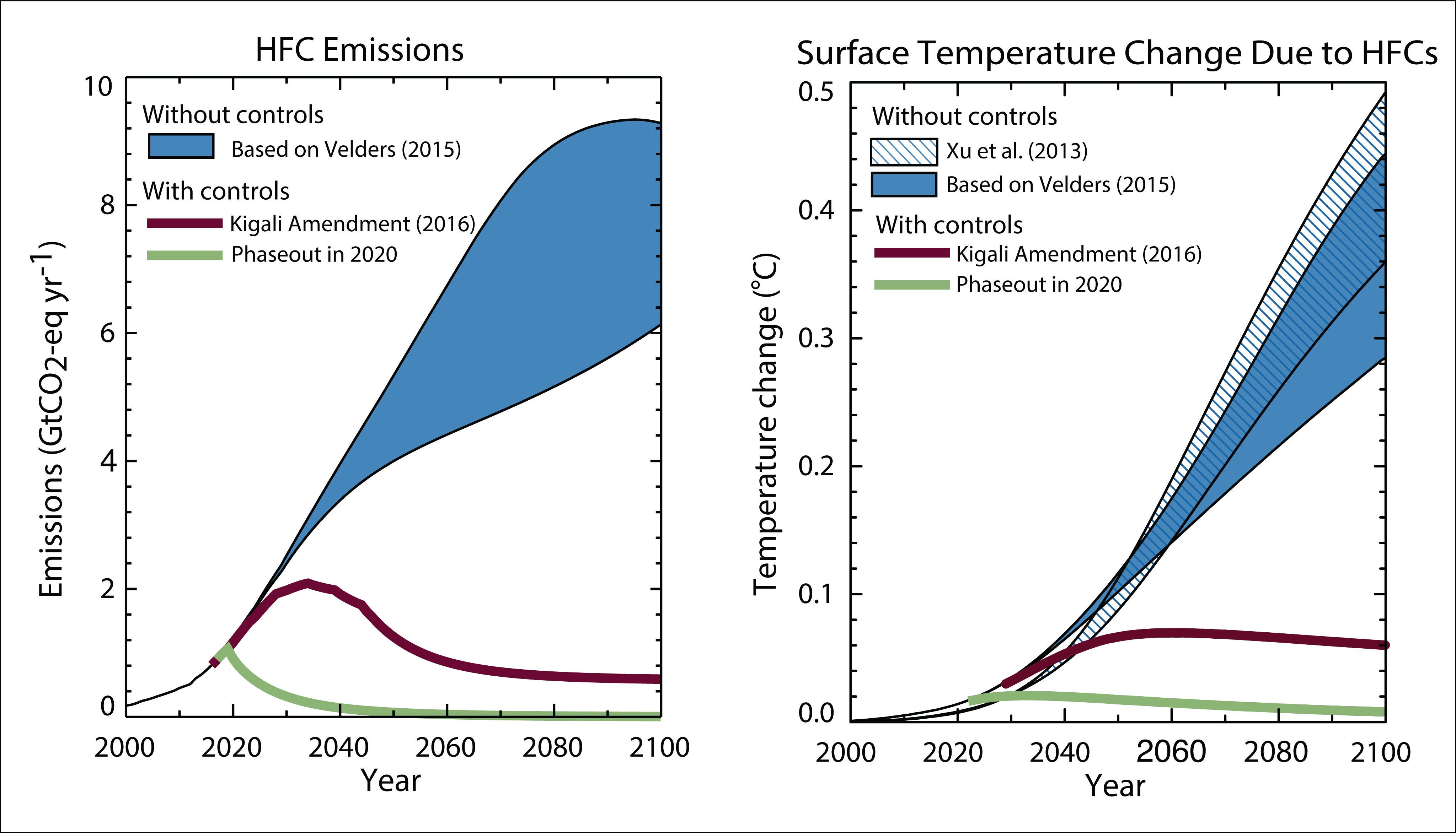
The Kigali Amendment is projected to reduce future global average warming in 2100 due to hydrofluorocarbons (HFCs) from a baseline of 0.3–0.5 °C to less than 0.1 °C. The magnitude of the avoided temperature increase due to the provisions of the Kigali Amendment (0.2 to 0.4 °C) is substantial in the context of the 2015 Paris Agreement, which aims to keep global temperature rise this century to well below 2 °C above pre-industrial levels. [ES Section 2]
There has been an unexpected increase in global total emissions of CFC-11. Global CFC-11 emissions derived from measurements by two independent networks increased after 2012, thereby slowing the steady decrease in atmospheric concentrations reported in previous Assessments. The global concentration decline over 2014 to 2016 was only two-thirds as fast as it was from 2002 to 2012. While the emissions of CFC-11 from eastern Asia have increased since 2012, the contribution of this region to the global emission rise is not well known. The country or countries in which emissions have increased have not been identified. [ES Section 1]
Sources of significant carbon tetrachloride emissions, some previously unrecognised, have been quantified. These sources include inadvertent by-product emissions from the production of chloromethanes and perchloroethylene, and fugitive emissions from the chlor-alkali process. The global budget of carbon tetrachloride is now much better understood than was the case in previous Assessments, and the previously identified gap between observation-based and industry-based emission estimates has been substantially reduced. [ES Sections 1 and 5]
Continued success of the Montreal Protocol in protecting stratospheric ozone depends on continued compliance with the Protocol. Options available to hasten the recovery of the ozone layer are limited, mostly because actions that could help significantly have already been taken. Remaining options such as complete elimination of controlled and uncontrolled emissions of substances such as carbon tetrachloride and dichloromethane; bank recapture and destruction of CFCs, halons, and HCFCs; and elimination of HCFC and methyl bromide production would individually lead to small-to-modest ozone benefits. Future emissions of carbon dioxide, methane, and nitrous oxide will be extremely important to the future of the ozone layer through their effects on climate and on atmospheric chemistry. Mitigation of nitrous oxide emissions would also have a small-to-modest ozone benefit. [Figure ES-9, ES Section 5]
Preface
This document contains information upon which the Parties to the Montreal Protocol on Substances that Deplete the Ozone Layer (“The Parties”) will base their future decisions regarding protection of the stratospheric ozone layer and climate from the production and consumption of ozone-depleting substances (ODSs) and their replacements.
The Charge to the Assessment Panels
Specifically, Article 6 of the Montreal Protocol on Substances that Deplete the Ozone Layer states:
Beginning in 1990, and at least every four years thereafter, the Parties shall assess the control measures provided for in Article 2 and Articles 2A to 2I on the basis of available scientific, environmental, technical and economic information.
To provide the mechanisms whereby these assessments are conducted, the Montreal Protocol further states:
“. . . the Parties shall convene appropriate panels of experts” and “the panels will report their conclusions . . . to the Parties.”
To meet this request, the Scientific Assessment Panel (SAP), the Environmental Effects Assessment Panel, and the Technology and Economic Assessment Panel each prepare, about every 3–4 years, major assessments that update the state of understanding in their purviews. These assessments are made available to the Parties in advance of their annual meetings at which they consider amendments and adjustments to the provisions of the Montreal Protocol.
Sequence of Scientific Assessments
The 2018 Assessment is the latest in a series of assessments prepared by the world’s leading experts in the atmospheric sciences and under the auspices of the Montreal Protocol in coordination with the World Meteorological Organization (WMO) and/or the United Nations Environment Programme (UN Environment). The 2018 Assessment is the ninth in the series of major assessments that have been prepared by the Scientific Assessment Panel as direct input to the Montreal Protocol process. The chronology of the nine scientific assessments of ozone depletion, along with other relevant reports and international policy decisions, are summarized in Table ES-1.
2018 Assessment Terms of Reference
The terms of reference of the 2018 Assessment were decided at the 27th Meeting of the Parties to the Montreal Protocol in Dubai, United Arab Emirates (1–5 November 2015) in their Decision XXVII/61:
5. To request the assessment panels to bring to the notice of the Parties any significant developments which, in their opinion, deserve such notice, in accordance with decision IV/13;
6. To request the Scientific Assessment Panel to undertake, in its 2018 report, a review of the scientific knowledge as dictated by the needs of the Parties to the Montreal Protocol, as called for in the terms of reference for the panels, taking into account those factors stipulated in Article 3 of the Vienna Convention, including estimates of the levels of ozone-layer depletion attributed to the remaining potential emissions of ozone-depleting substances and an assessment of the level of global emissions of ozone depleting substances below which the depletion of the ozone layer could be comparable to various other factors such as the natural variability of global ozone, its secular trend over a decadal timescale and the 1980 benchmark level;
and in their Decision XXVII/72:
7. To request the Technology and Economic Assessment Panel and the Scientific Assessment Panel to continue their analysis of the discrepancies between observed atmospheric concentrations and reported data on carbon tetrachloride and to report and provide an update on their findings to the Twenty-Eighth Meeting of the Parties.
Significant developments since the 2014 Assessment that are included in the 2018 Assessment are (i) the adoption of the Kigali Amendment in 2016 to phase down global hydrofluorocarbon (HFC) production and consumption; (ii) the recognition of increased global emissions of CFC-11; and (iii) an improved understanding of the budget of carbon tetrachloride (CCl4).
The Assessment Process
The process of writing the current Assessment started early in 2016. The SAP co-chairs considered suggestions from the Parties regarding experts from their countries who could participate in the process. Further, an ad hoc international scientific advisory group was formed to suggest authors and reviewers from the world scientific community and to help craft the Assessment outline. As in previous Assessments, the participants represented experts from the developed and developing world who bring a special perspective to the process and whose involvement in the Assessment contributes to capacity building. The Appendix provides a listing of the approximately 280 scientists from 31 countries who contributed to the preparation and review of the Assessment.
An initial letter was sent to a large number of scientists and policy makers in November 2016 soliciting comments and inputs on a draft outline along with suggestions for authors for the 2018 Assessment. This was followed by revisions to the outline and recruitment of lead authors and co-authors. The steering committee and lead authors met in London, UK, in May 2017 to review the revised chapter outlines. The chapter writing process produced five drafts between mid-September 2017 and August 2018 aided by two author team meetings (Boulder, Colorado, USA and Les Diablerets, Switzerland). The first and third drafts were formally peer-reviewed by a large number of expert reviewers. The chapters were revised by the author teams based on the extensive review comments (numbering over 5000) and the review editors for each chapter provided oversight of the revision process to ensure that all comments were addressed appropriately.
At a meeting in Les Diablerets, Switzerland, held on 16–20 July 2018, the Executive Summary contained herein was prepared and completed by the 68 attendees of the meeting. These attendees included the steering committee, chapter lead authors, review editors, some chapter co-authors (selected by the chapter leads), reviewers (selected by the review editors), and some leading experts invited by the steering committee. The Executive Summary, initially drafted by the Assessment steering committee, was reviewed, revised, and approved line-by-line. The Highlights section was drafted during the meeting to provide a concise summary of the Executive Summary.
The success of the 2018 Assessment depended on the combined efforts and commitment of a large international team of scientific researchers who volunteered their time as lead authors, contributors, reviewers, and review editors and on the skills and dedication of the assessment coordinator and the editorial and production staff, who are listed at the end of this report.
Table ES-1. Chronology of scientific reports and policy decisions related to ozone depletion.
| Year | Policy Decisions | Scientific Reports |
|---|---|---|
| 1981 | The Stratosphere 1981: Theory and Measurements. WMO No. 11. | |
| 1985 | Vienna Convention | Atmospheric Ozone 1985. Three volumes. WMO No. 16. |
| 1987 | Montreal Protocol | |
| 1988 | International Ozone Trends Panel Report 1988. Two volumes. WMO No. 18. | |
| 1989 | Scientific Assessment of Stratospheric Ozone: 1989. Two volumes. WMO No. 20. | |
| 1990 | London Adjustment and Amendment | |
| 1991 | Scientific Assessment of Ozone Depletion: 1991. WMO No. 25. | |
| 1992 | Methyl Bromide: Its Atmospheric Science, Technology, and Economics (Montreal Protocol Assessment Supplement). UNEP (1992) | |
| 1992 | Copenhagen Adjustment and Amendment | |
| 1994 | Scientific Assessment of Ozone Depletion: 1994. WMO No. 37. | |
| 1995 | Vienna Adjustment | |
| 1997 | Montreal Adjustment and Amendment | |
| 1998 | Scientific Assessment of Ozone Depletion: 1998. WMO No. 44. | |
| 1999 | Beijing Adjustment and Amendment | |
| 2002 | Scientific Assessment of Ozone Depletion: 2002. WMO No. 47. | |
| 2006 | Scientific Assessment of Ozone Depletion: 2006. WMO No. 50. | |
| 2007 | Montreal Adjustment | |
| 2010 | Scientific Assessment of Ozone Depletion: 2010. WMO No. 52. | |
| 2014 | Scientific Assessment of Ozone Depletion: 2014. WMO No. 55. | |
| 2016 | Kigali Amendment | |
| 2018 | Scientific Assessment of Ozone Depletion: 2018. WMO No. 58. |
Introduction
The 1985 Vienna Convention for the Protection of the Ozone Layer is an international agreement in which United Nations States recognized the fundamental importance of preventing damage to the stratospheric ozone layer. The 1987 Montreal Protocol on Substances that Deplete the Ozone Layer and its succeeding amendments, adjustments, and decisions were subsequently negotiated to control the consumption and production of anthropogenic ozone-depleting substances (ODSs) and some hydrofluorocarbons (HFCs). The Montreal Protocol Parties base their decisions on scientific, environmental, technical, and economic information that is provided by their technical panels. The Protocol requests quadrennial reports from its Scientific Assessment Panel that update the science of the ozone layer. This Executive Summary (ES) highlights the key findings of the Scientific Assessment of Ozone Depletion: 2018, as put together by an international team of scientists. The key findings of each of the six chapters of the Scientific Assessment have been condensed and formulated to make the ES suitable for a broad audience.
Ozone depletion is caused by human-related emissions of ODSs and the subsequent release of reactive halogen gases, especially chlorine and bromine, in the stratosphere. ODSs include chlorofluorocarbons (CFCs), bromine-containing halons and methyl bromide, hydrochlorofluorocarbons (HCFCs), carbon tetrachloride (CCl4), and methyl chloroform. The substances controlled under the Montreal Protocol are listed in the various annexes to the agreement (CFCs and halons under Annex A and B, HCFCs under Annex C, and methyl bromide under Annex E)3. These ODSs are long-lived (e.g., CFC-12 has a lifetime greater than 100 years) and are also powerful greenhouse gases (GHGs). As a consequence of Montreal Protocol controls, the stratospheric concentrations of anthropogenic chlorine and bromine are declining.
In addition to the longer-lived ODSs, there is a broad class of chlorine- and bromine-containing substances known as very short-lived substances (VSLSs) that are not controlled under the Montreal Protocol and have lifetimes shorter than about 6 months. For example, bromoform (CHBr3) has a lifetime of 24 days, while chloroform (CHCl3) has a lifetime of 149 days. These substances are generally destroyed in the lower atmosphere in chemical reactions. In general, only small fractions of VSLS emissions reach the stratosphere where they contribute to chlorine and bromine levels and lead to increased ozone depletion.
The Montreal Protocol’s control of ODSs stimulated the development of replacement substances, firstly HCFCs and then HFCs, in a number of industrial sectors. While HFCs have only a minor effect on stratospheric ozone, some HFCs are powerful GHGs. Previous Assessments have shown that HFCs have been increasing rapidly in the atmosphere over the last decade and were projected to increase further as global development continued in the coming decades. The adoption of the 2016 Kigali Amendment to the Montreal Protocol (see Annex F) will phase down the production and consumption of some HFCs and avoid much of the projected global increase and associated climate change.
Observations of atmospheric ozone are made by instruments on the ground and on board balloons, aircraft, and satellites. This network of observations documented the decline of ozone around the globe, with extreme depletions occurring over Antarctica in each spring and occasional large depletions in the Arctic, and they allowed us to report some indications of recovery in stratospheric ozone in the 2014 Assessment. The chemical and dynamical processes controlling stratospheric ozone are well understood, with ozone depletion being fundamentally driven by the atmospheric abundances of chlorine and bromine.
Previous Assessments have shown projections of decreasing ODSs, and models show that global ozone should increase as a result. Models have also demonstrated that increasing concentrations of the GHGs carbon dioxide (CO2) and methane (CH4) during this century will cause global ozone levels to increase beyond the natural level of ozone observed in the 1960s, primarily because of the cooling of the upper stratosphere and a change of the stratospheric circulation. On the other hand, the chemical effect of increasing concentrations of nitrous oxide (N2O), another GHG, will be to deplete stratospheric ozone.
This 2018 Assessment is the ninth in a series that is provided to the Montreal Protocol by its Scientific Assessment Panel. In this Assessment, many of our previous Assessment findings are strengthened and new results are presented. A clear message of the 2018 Assessment is that the Montreal Protocol continues to be effective at reducing the atmospheric abundance of ODSs.
Executive Summary
[1] Concentrations and trends in ozone-depleting substances (ODSs)
Total chlorine and total bromine
Our confidence that the Montreal Protocol is continuing to work is based on a sustained network of measurements of the long-lived source gas concentrations over several decades. These measurements allow the determination of global concentrations, their interhemispheric differences, and their trends. Combined with lifetime information, the data allow us to derive historical emissions which can be compared with emissions derived from data reported to UN Environment.
The atmospheric abundances of both total tropospheric chlorine and total tropospheric bromine from long-lived ODSs controlled under the Montreal Protocol have continued to decline since the 2014 Assessment (Figure ES-1, panels a, b; Table ES-2).
During the period 2012–2016, the observed rate of decline in tropospheric chlorine due to controlled substances was 12.7 ± 0.9 ppt Cl yr−1, which is very close to the baseline projection from the 2014 Assessment. The net rate of change was the result of a slower than projected decrease in CFC concentrations and a slower than projected increase in HCFCs relative to the 2014 scenario. That scenario was based on the maximum allowed production of HCFCs from Article 5 countries under the Montreal Protocol.
The decrease of chlorine from controlled substances has partly been offset by increases in the mainly natural CH3Cl and mainly anthropogenic very short-lived gases, which are not controlled under the Montreal Protocol.
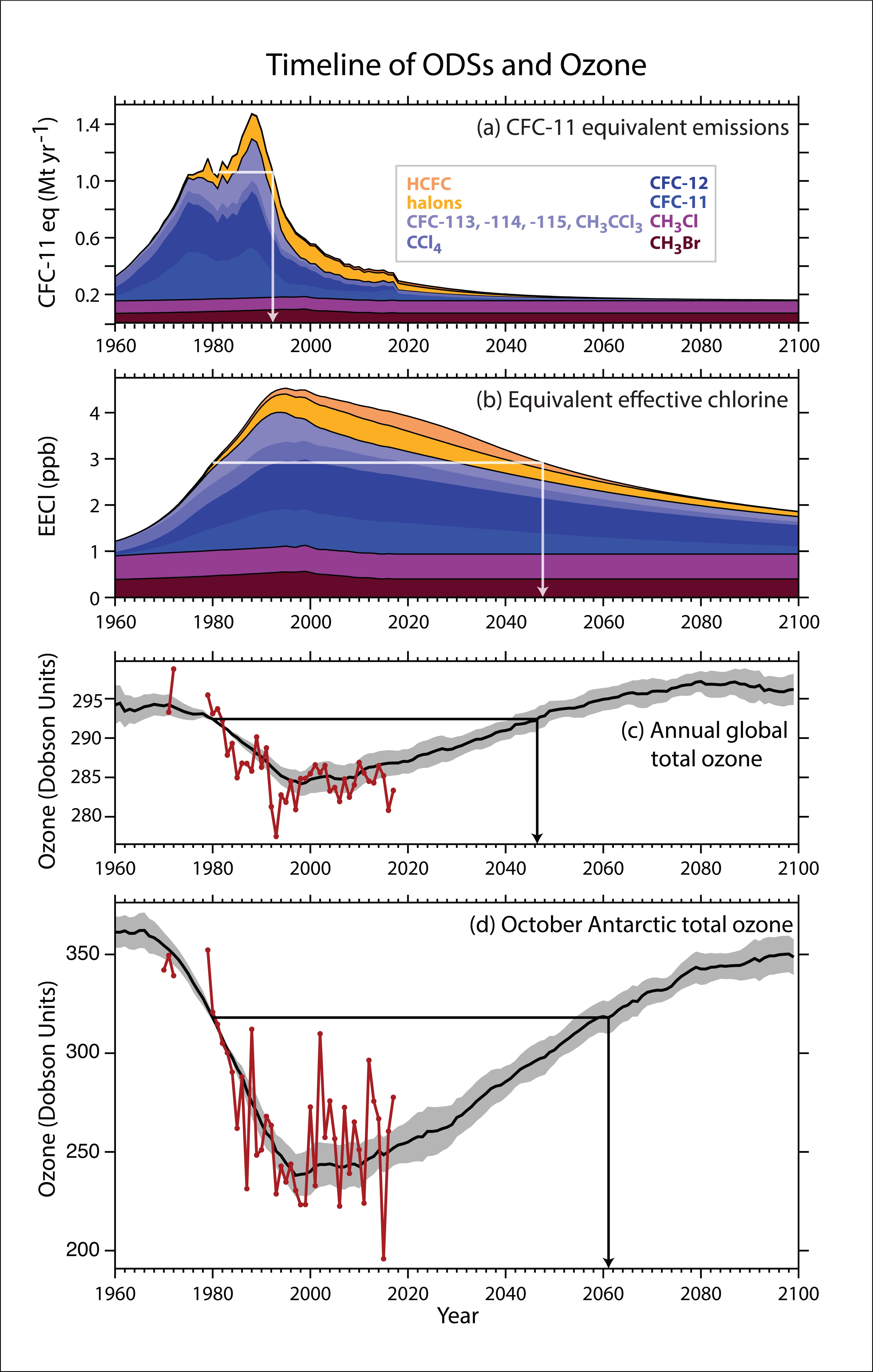
Table ES-2. Contributions of various long-lived ozone-depleting substances controlled under the Montreal Protocol to tropospheric organic chlorine and bromine in 2016, and annual average trends between 2012 and 2016.
| Contribution to tropospheric chlorine and bromine in 20161 (ppt Cl/Br) | Changes in tropospheric chlorine and bromine (in parts per trillion (ppt) (Cl/Br) yr-1) from early-2012 to late-2016 | |
|---|---|---|
| Controlled chlorine substances by group | ||
| chlorofluorocarbons (CFCs) | 1979 | −12.0 ± 0.4 |
| methyl chloroform (CH3CCl3) | 7.8 | −2.0 ± 0.5 |
| carbon tetrachloride (CCl4) | 322 | −4.5 ± 0.2 |
| hydrochlorofluorocarbons (HCFCs) | 309 | +5.9 ± 1.3 |
| halon-1211 | 3.6 | −0.1 ± 0.01 |
| Total Chlorine from controlled substances | 2621 | −12.7 ± 0.9 |
| Controlled bromine substances by group | ||
| halons | 7.8 | −0.1 ± 0.01 |
| methyl bromide (CH3Br)2 | 6.8 | −0.04 ± 0.05 |
| Total bromine from controlled substances | 14.6 | −0.15 ± 0.04 |
1 Values are annual averages.
2 Not all CH3Br emissions are controlled. Some anthropogenic uses of CH3Br are exempted from Montreal Protocol controls, and CH3Br has natural sources, which results in a natural background concentration.
Unexpected increase in global total emissions of CFC-11
Observations of the persistent slowdown in the decline of CFC-11 concentrations have only recently allowed the robust conclusion that emissions of CFC-11 have increased in recent years, as opposed to other possible causes for the slowdown such as changing atmospheric circulation.
Global CFC-11 emissions, derived from measurements by two independent networks, increased after 2012 contrary to projections from previous Assessments, which showed decreasing emissions (Figure ES-2). This conclusion is supported by the observed rise in the CFC-11 hemispheric concentration difference. Global CFC-11 emissions for 2014 to 2016 were approximately 10 Gg yr-1 (about 15%) higher than the fairly constant emissions derived for 2002 to 2012; the excess emissions relative to projected emissions for recent years is even larger. The increase in global emissions above the 2002–2012 average resulted in a global concentration decline in CFC-11 over 2014 to 2016 that was only two-thirds as fast as from 2002 to 2012.
The CFC-11 emission increase suggests new production not reported to UN Environment because the increase is inconsistent with likely changes in the release of CFC-11 from banks associated with pre-phaseout production. Depending on how this newly produced CFC-11 is being used, substantial increases in the bank and future emissions are possible.
Emissions of CFC-11 from eastern Asia have increased since 2012; the contribution of this region to the global emission rise is not well known. The country or countries in which emissions have increased have not yet been identified.

Persistent emissions of low abundance CFCs
Observation-based analyses show unexpected stable or even increasing emissions of some of the low abundance (less than 20 ppt) CFCs (CFC-13, CFC-113a, CFC-114, CFC-115) between 2012 and 2016. For CFC-114 and CFC-115, atmospheric observations imply that a substantial fraction of global emissions originated from China.
Ongoing substantial emissions of carbon tetrachloride (CCl4)
Sources of significant CCl4 emissions, some previously unrecognized, have been quantified. At least 25 Gg yr-1 of emissions have been estimated, mainly originating from the industrial production of chloromethanes, perchloroethylene and chlorine. This value can be compared with total global emissions of approximately 35 Gg yr-1, derived from atmospheric observations. The global CCl4 budget is now much better understood and the previously identified gap between observation-based and industry-based emission estimates has been substantially reduced compared to the 2014 Assessment.
Hydrochlorofluorocarbons (HCFCs)
-
Total chlorine from HCFCs has continued to increase in the atmosphere since the last Assessment and reached 309 ppt in 2016. The annual average growth rate of chlorine from HCFCs decreased from 9.2 ± 0.3 ppt yr-1 for the 2008 to 2012 period to 5.9 ± 1.3 ppt yr-1 for the 2012 to 2016 period.
-
Combined emissions of the major HCFCs have declined since the last Assessment which suggests an effective response to the 2007 Adjustment to the Montreal Protocol that limited HCFC emissions. Annual emissions of HCFC-22 have remained relatively unchanged since 2012, whilst emissions of HCFC-141b and-142b declined by around 10% and 18%, respectively, between 2012 and 2016. These findings are consistent with a decrease in reported HCFC consumption after 2012, particularly from Article 5 countries.
Tropospheric bromine
Total tropospheric bromine from controlled ODSs (halons and methyl bromide) continued to decrease and by 2016 was 14.6 ppt, 2.3 ppt below the peak levels observed in 1998. In the 4-year period prior to the last Assessment, this decrease was primarily driven by a decline in methyl bromide (CH3Br) abundance, with a smaller contribution from a decrease in halons. These relative contributions have now reversed, with halons being the main driver of the decrease of 0.15 ± 0.04 ppt yr−1 tropospheric bromine between 2012 and 2016.
Total bromine from halons has decreased from a peak of 8.5 ppt in 2005 to 7.7 ppt in 2016. Emissions of halons derived from atmospheric observations declined or remained stable between 2012 and 2016 and are thought to originate primarily from banks.
The atmospheric abundance of CH3Br declined from a peak of 9.2 ppt in 1996–1998 to 6.8 ppt in 2016 as a consequence of controls under the Montreal Protocol. By 2016, controlled CH3Br consumption had declined by more than 98% from its peak value. Reported consumption in quarantine and pre-shipment (QPS) uses of CH3Br, which are not controlled under the Montreal Protocol, has not changed substantially over the last two decades. Total reported anthropogenic emissions (controlled and not-controlled) have declined by about 85% from the peak value, and atmospheric CH3Br abundance is now near the expected natural background.
Halogenated very short-lived substances (VSLSs)
Halogenated VSLS substances contribute to stratospheric chlorine and bromine loading and are not controlled by the Montreal Protocol. Chlorinated VSLSs are predominantly of anthropogenic origin, while brominated VSLSs have mainly natural sources.
Dichloromethane (CH2Cl2) is the main component of VSLS chlorine and accounts for the majority of the rise in total chlorine from VSLSs between 2012 and 2016. A substantial fraction of the global CH2Cl2 emissions has been attributed to southern and eastern Asia. The current estimate is that total chlorine from VSLS source gases increased by about 20 ppt between 2012 and 2016 to reach 110 ppt (Figure ES-3). The growth rate shows large interannual variability.
Several field campaigns conducted since the last Assessment have confirmed that brominated VSLSs contribute 5±2 ppt to stratospheric bromine (Figure ES-3). There is no indication in measurements of a long-term trend in the contribution of VSLSs to stratospheric bromine.
Total stratospheric chlorine and bromine
Total stratospheric chlorine and bromine both continue to decline. Even though the abundance of bromine is much smaller than that of chlorine, bromine has a significant impact because it is around 60–65 times more efficient than chlorine in destroying ozone.
Total chlorine entering the stratosphere from well-mixed ODSs declined by 405 ppt (12%) between the 1993 peak (3582 ppt) and 2016 (3177 ppt). (Figure ES-3) This decline was driven by decreasing atmospheric abundances of methyl chloroform (CH3CCl3), CFC-11 and CCl4 (in order of importance). The VSLS contribution (primarily anthropogenic) has increased over this period but remains below 4% of the total in 2016. About 80% of the chlorine entering the stratosphere annually is of anthropogenic origin.
Total bromine entering the stratosphere from well-mixed ODSs declined by 2.4 ppt (15%) between the 1998 peak (16.9 ppt) and 2016 (14.5 ppt). (Figure ES-3) This decline was driven by decreasing atmospheric abundances of methyl bromide (CH3Br), halon-1211, and halon 2402 (in order of importance). The VSLS (primarily biogenic) contribution has no measurable change over this period, contributing about 25% to the total in 2016. The natural components of CH3Br and VSLSs now contribute more than half of the bromine entering the stratosphere annually.
HCl is the major chlorine component in the upper stratosphere. Its concentration in this region decreased by about 6% between 2005 and 2016. This decrease is consistent with the decline in total chlorine entering the stratosphere.
Total stratospheric bromine derived from bromine monoxide (BrO) observations decreased by about 8% from 2004 to 2014. This decrease is consistent with the decline in total bromine entering the stratosphere.

[2] Hydrofluorocarbons (HFCs)
The Montreal Protocol phaseout of ODSs has led to the development of alternative substances for use in many sector applications. Hydrofluorocarbons (HFCs) are a widely used category of ODS alternatives that do not contain ozone-depleting chlorine or bromine. Long-lived CFCs, HCFCs, and HFCs are all potent greenhouse gases. Ultimately the Kigali Amendment to the Montreal Protocol, which was adopted in 2016 and will come into force in 2019, sets schedules for the phasedown of global production and consumption of specific HFCs. Although the radiative forcing supplied by atmospheric HFC abundances is currently small, the Kigali Amendment is designed to avoid unchecked growth in emissions and associated warming in response to projected increasing demand in coming decades. Discussed here are the anticipated overall effects of Kigali Amendment controls and existing national and regional HFC regulations on future HFC abundances and associated climate warming. HFCs were included as one group within the basket of gases of the 1997 Kyoto Protocol and, as a result, developed (Annex-I) countries supply annual emission estimates of HFCs to the United Nations Framework Convention on Climate Change (UNFCCC). HFC-23 is considered separately in the Kigali Amendment and in this Assessment, primarily because it is emitted to the atmosphere as a by-product of HCFC-22 production. HFC-23 has one of the longest atmospheric lifetimes and highest global warming potentials (GWP) among HFCs. HFC-23 is not included in the projections discussed here.
Observed HFC abundances and associated emissions
Atmospheric abundances of most currently measured HFCs are increasing in the global atmosphere. These increases are similar to those projected in the baseline scenario of the 2014 Assessment. HFC emissions derived from observations increased by 23% from 2012 to 2016 and currently amount to about 1.5% of total emissions from all long-lived greenhouse gases as carbon dioxide-equivalent emissions (GtCO2-eq).
HFC emissions estimated from the combination of inventory reporting and atmospheric observations indicate that the HFC emissions originate from both developed and developing countries. Only developed (Annex I) countries are required to report HFC emissions to the UNFCCC, and these reported totals account for less than half of global emissions (as CO2-eq) derived from observations.
Radiative forcing from measured HFCs continues to increase; it currently amounts to 1% (0.03 W m-2) of the 3 W m-2 supplied by all long-lived greenhouse gases (GHGs) including CO2, CH4, N2O, and halocarbons. Total HFC radiative forcing in 2016 was about 10% of the 0.33 W m-2 supplied by all halocarbons.
Global annual emissions of HFC-23, a potent greenhouse gas and a byproduct of HCFC-22 production, have varied substantially in recent years. This variability in observationally derived global emissions is broadly consistent with the sum of reported HFC-23 emissions associated with HCFC-22 production from developed countries and inventory-based estimates of HFC-23 emissions from developing countries. Future HFC-23 emission trends will largely depend on the magnitude of HCFC-22 production and the effectiveness of HFC-23 destruction associated with that production.
Some short-lived, low-GWP replacement substances for long-lived HCFCs and HFCs have been detected in the atmosphere (at concentrations typically below 1 ppt), consistent with the transition to these substances being underway. Some of these substances are unsaturated HCFCs and unsaturated HFCs, also known as hydrofluoroolefins or HFOs.
Projections of HFC emissions and temperature contributions
The HFC phasedown schedule of the 2016 Kigali Amendment to the Montreal Protocol substantially reduces future projected global HFC emissions (Figure ES-4). Emissions are projected to peak before 2040 and decline to less than 1 GtCO2-eq yr-1 by 2100 (Figure ES-4). Only marginal increases are projected for CO2-eq emissions of the low-GWP alternatives (Figure ES-5) despite substantial projected increases in their emission mass.
The Kigali Amendment, assuming global compliance, is projected to reduce future radiative forcing due to HFCs by about 50% in 2050 compared to a scenario without any HFC controls. The estimated benefit of the amendment is the avoidance of 2.8 - 4.1 GtCO2-eq yr-1 emissions by 2050 and 5.6 - 8.7 GtCO2-eq yr-1 by 2100. For comparison, total CH4 emissions are projected to be 7 - 25 GtCO2-eq yr-1 by 2100 in the RCP-6.0 and RCP-8.5 scenarios and total N2O emissions 5-7 GtCO2-eq yr-1 by 2100.
The Kigali Amendment is projected to reduce future global average warming in 2100 due to HFCs from a baseline of 0.3-0.5 °C to less than 0.1 °C (Figure ES-4). If the global production of HFCs were to cease in 2020, the surface temperature contribution of the HFC emissions would stay below 0.02 °C for the whole 21st century. The magnitude of the avoided temperature increase, due to the provisions of the Kigali Amendment (0.2 to 0.4 °C) is substantial in the context of the 2015 UNFCCC Paris Agreement, which aims to limit global temperature rise to well below 2.0 °C above pre-industrial levels and to pursue efforts to limit the temperature increase even further to 1.5 °C.
[3] Stratospheric ozone
The Montreal Protocol and its Amendments and Adjustments have been effective in limiting the abundance of ODSs in the atmosphere. Detecting and attributing ozone trends during this period of slow ODS decline is challenging because of large natural variability in ozone, as well as confounding factors such as climate change and changes in tropospheric ozone. While most natural variability is quasi-periodic, episodic volcanic eruptions can drive large changes in ozone in the presence of elevated halogen abundances. The Antarctic and the upper stratosphere, where the ozone depletion signal has been clearest against the backdrop of natural variability, are now showing evidence of recovery. Although the Arctic stratosphere is warmer and experiences much more meteorological variability, severe chemical ozone loss can occur when cold conditions persist into March/April (Figure ES-6). Ozone in the tropical lower stratosphere shows little response to changes in ODSs, because halogen-driven ozone depletion is small in this region.
Antarctic and Arctic ozone
-
For the first time, there are emerging indications that the Antarctic ozone hole has diminished in size and depth since the year 2000, with the clearest changes occurring during early spring. Although accounting for natural variability is challenging, the weight of evidence suggests that the decline in ODSs made a substantial contribution to the observed trends.
-
Even with these early signs of recovery, an Antarctic ozone hole continues to occur every year, with the severity of the chemical loss strongly modulated by meteorological conditions (temperatures and winds) (Figure ES-1). In 2015, the ozone hole was particularly large and long-lasting, as a result of a cold and undisturbed polar stratospheric vortex. Aerosols from the Calbuco volcanic eruption are also believed to have contributed to the large ozone hole area in 2015. Conversely, in 2017, the Antarctic ozone hole was very small due to a warm and unusually disturbed polar vortex.
-
In the Arctic, year-to-year variability in column ozone is much larger than in the Antarctic, precluding identification of a statistically significant4 increase in Arctic ozone over the 2000–2016 period. Exceptionally low ozone abundances, similar to those experienced in Arctic spring 2011, have not bee observed in the last four years. Extremely cold conditions in the 2015/2016 winter resulted in rapid chemical ozone loss, but a sudden warming of the polar stratosphere in early March curtailed further losses.
-
Model simulations show that implementation of the Montreal Protocol has prevented much more severe ozone depletion than has been observed in the polar regions of both hemispheres (Figure ES-6).

Global ozone
-
No statistically significant trend has been detected in global (60°S–60°N) total column ozone over the 1997–2016 period (Figure ES-1). Average global total column ozone in the years since the last Assessment remain roughly 2.2% below the 1964–1980 average. These findings are expected given our understanding of the processes that control ozone.
-
In the mid-latitudes, the increase in ozone expected to arise from the 15% decline in EESC since 1997 is small (1% per decade) relative to the year-to-year variability (about 5%).
-
In the tropics, where halogen-driven ozone loss is small in the lower stratosphere, total column ozone has not varied significantly with ODS concentrations, except under conditions of high volcanic aerosol loading (e.g., Mt. Pinatubo).
-
Upper stratospheric ozone, which represents only a small fraction of the total column, has increased by 1–3% per decade since 2000 outside of polar regions (Figure ES-7). Additional and improved data sets and focused studies evaluating trend uncertainties have strengthened our ability to assess ozone profile changes since the last Assessment. The upward trend is largest and statistically significant in northern mid-latitudes and maximizes above 40-km altitude.
Model simulations attribute about half of the observed upper stratospheric ozone increase after 2000 to the decline of ODSs since the late 1990s.
The other half of the ozone increase is attributed to the slowing of gas-phase ozone destruction, which results from cooling of the upper stratosphere caused by increasing GHGs.
-
There is some evidence for a decrease in global (60°S–60°N) lower stratospheric ozone from 2000 to 2016, but it is not statistically significant in most analyses. Much of the apparent decline in the tropics and mid-latitudes was reversed by an abrupt increase in ozone in 2017, showing that longer records are needed to identify robust trends. Model simulations indicate that, on multiannual timescales, variations in ozone in this region are primarily controlled by transport rather than chemistry.

Ozone recovery and ozone-climate interactions
A refined ODS scenario and new GHG emissions scenarios were used in chemistry-climate models for this Assessment, leading to a delay of about 5 to 15 years in the return dates relative to the last Assessment, depending on the latitude region.
-
Updated chemistry climate model projections based on full compliance with the Montreal Protocol and assuming the baseline estimate of the future evolution of GHGs (RCP-6.0) show that:
The Antarctic ozone hole is expected to gradually close, with springtime total column ozone returning to 1980 values shortly after mid-century (about 2060) (Figure ES-1);
Arctic springtime total ozone is expected to return to 1980 values before mid-century (about 2030s). Substantial Arctic ozone loss will remain possible in cold winters as long as ODS concentrations are well above natural levels. In contrast to the Antarctic, the timing of the recovery of Arctic total ozone in spring will be strongly affected by anthropogenic climate change;
Northern-Hemisphere, mid-latitude column ozone is expected to return to 1980 abundances before mid-century (2030s), and Southern Hemisphere, mid-latitude ozone is expected to return around mid-century.
-
Outside the Antarctic, CO2, CH4, and N2O will be the main drivers of stratospheric ozone changes in the second half of the 21st century, assuming full compliance with the Montreal Protocol. These gases impact both chemical cycles and the stratospheric overturning circulation, with a larger response in stratospheric ozone associated with stronger climate forcing. By 2100 the stratospheric column is expected to:
decrease in the tropics by about 5 DU for RCP-4.5 and about 10 DU for RCP-8.5, with the net total column change projected to be smaller (about 5 DU) because of offsetting increases in tropospheric ozone; and
not only to recover but to exceed 1960–1980 average values in mid-latitudes and the Arctic, with springtime Arctic ozone being higher by about 35 DU for RCP-4.5 and about 50 DU for RCP-8.5.
[4] Ozone change and its influence on climate
Ozone is important in the climate system and its changes can influence both the troposphere and the stratosphere. Past Assessments have discussed evidence for how stratospheric ozone depletion has affected Southern Hemisphere climate. The climate impacts of ozone depletion are expected to reverse over coming decades as stratospheric ozone recovers. However, projected increases in atmospheric GHG concentrations will continue to be a key driver of future Southern Hemisphere climate. The relative importance of ozone recovery for future Southern Hemisphere climate will depend on the evolution of atmospheric GHG concentrations.
Influence on stratospheric climate
Discrepancies between estimates of stratospheric cooling rates from different satellite temperature retrievals have been substantially reduced since the last Assessment. This result has led to greater confidence in the attribution of observed stratospheric temperature changes since the late 1970s.

Decreases in stratospheric ozone caused by ODS increases have been an important contributor to observed stratospheric cooling. New studies find that ODSs thereby contributed approximately one third of the observed cooling in the upper stratosphere from 1979 to 2005, with two thirds caused by increases in other GHGs.
Satellite temperature records show weaker global-average cooling throughout the depth of the stratosphere between 1998 and 2016 relative to between 1979 and 1997. The difference in the rate of stratospheric cooling between the two periods is consistent with differences in the observed ozone trends for each period.
Influence on surface climate and oceans
New studies strengthen the conclusion from the last Assessment that lower stratospheric cooling due to ozone depletion has very likely been the dominant cause of late 20th century changes in Southern Hemisphere climate in summer. These changes include the observed poleward shift in Southern Hemisphere tropospheric circulation, with associated impacts on surface temperature and precipitation (Figure ES-8). No robust link between stratospheric ozone depletion and long-term surface climate changes in the Northern Hemisphere has been established.
Changes in tropospheric circulation driven by ozone depletion have contributed to recent trends in Southern Ocean temperature and circulation; the impact on Antarctic sea ice remains unclear.
New studies since the last Assessment have not found a causal link between ozone depletion and the net strength of the Southern Ocean carbon sink over the last few decades. This result updates the 2010 Assessment where such a link was suggested.
[5] Policy considerations for stratospheric ozone and climate
Policy-relevant alternative scenarios related to future ozone changes
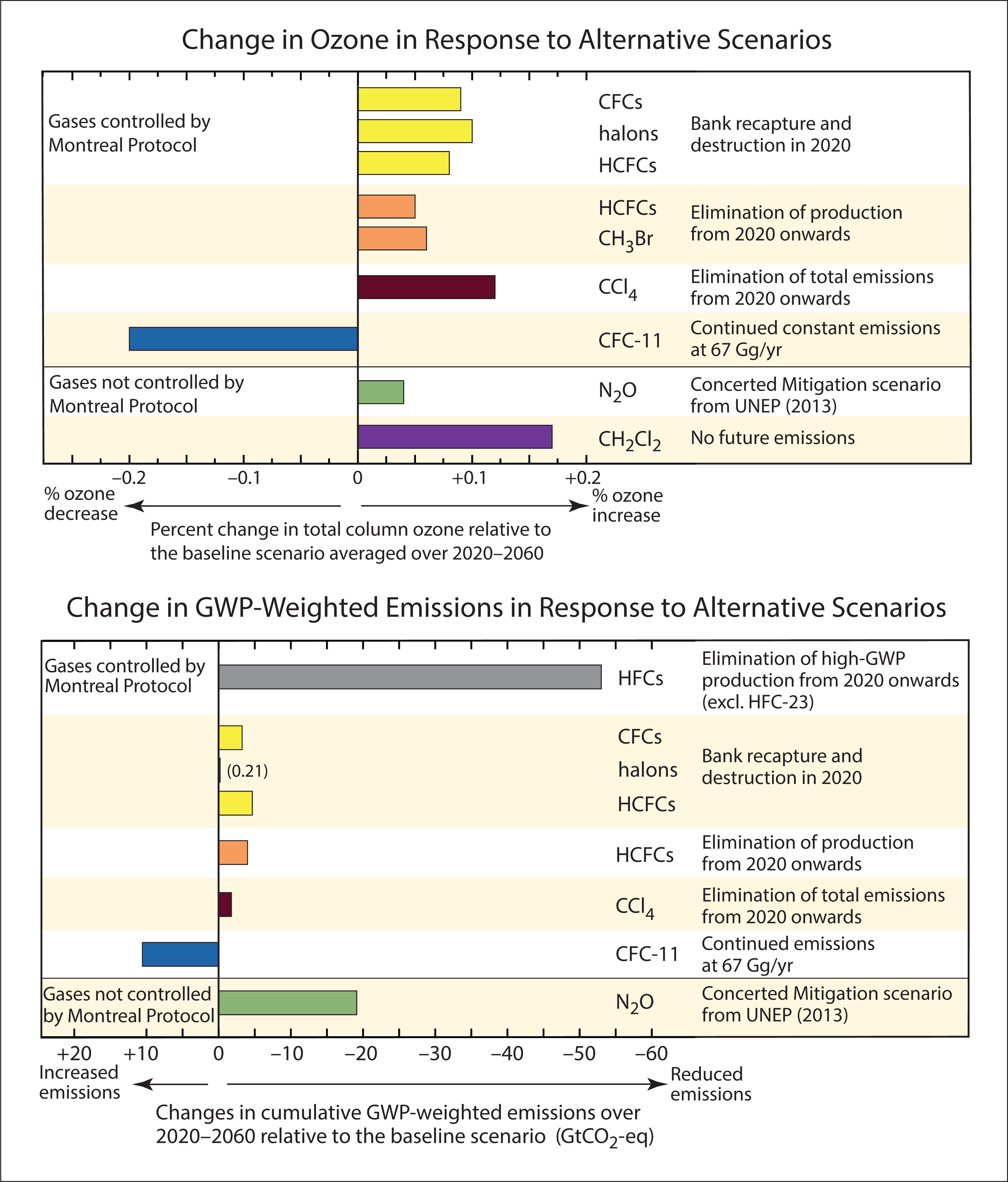
Changes in total column ozone and GWP-weighted emissions in response to various control measures and alternative scenarios are shown in Figure ES-9. The baseline scenario used here and those used in previous Assessments assume compliance with the Montreal Protocol. The alternative scenarios assessed here include the elimination of banks, production, and emissions of gases that are both controlled and uncontrolled by the Montreal Protocol. Key conclusions are found in the bullet points below.
The recently derived increase in global emissions of CFC-11 (Figure ES-2, Section 1) indicates that there is global production that is not reported to UN Environment. Assuming total emissions of CFC-11 continue at their average level from 2002–2016 (67 Gg yr-1), the return of mid-latitude and polar EESC values to their 1980 values would be delayed by about 7 and 20 years, respectively, compared to the recovery date expected from the continued declining bank emissions expected from the baseline scenario in which no unreported production is considered. Avoiding this scenario (blue bar in top panel of Figure ES-9) would have a larger positive impact on future ozone than any of the other mitigation options considered in Figure ES-9.
Future emissions from ODS banks continue to be a slightly larger contributor than future ODS production to ozone layer depletion over the next four decades in the baseline scenario. The baseline scenarios assume compliance with the Montreal Protocol. Future emissions from the banks of halons, CFCs, and HCFCs are projected to contribute roughly comparable amounts to EESC over the next few decades.
CCl4 emissions inferred from atmospheric observations continue to be much greater than those assumed from feedstock uses as reported to UN Environment. A significant part of these additional emissions has been identified as inadvertent by-product emissions from chloromethanes and perchloroethylene plants and fugitive emissions from the chlor-alkali process. Elimination of all CCl4 emissions in 2020 would accelerate the return of mid-latitude EESC to 1980 levels by almost three years.
Elimination of future quarantine and pre-shipment (QPS) production of methyl bromide (CH3Br) would accelerate the return of mid-latitude EESC to 1980 levels by about a year. Production for QPS applications is not controlled by the Montreal Protocol. QPS has remained nearly unchanged over the last two decades, and now constitutes almost 90% of the reported production of CH3Br because of the phaseout of other uses.
A number of gases of anthropogenic origin that are not controlled by the Montreal Protocol can have direct chemical effects on stratospheric ozone, for example dichloromethane (CH2Cl2) and N2O.
Emissions of anthropogenic VSLS chlorine contribute to ozone depletion. Observed growth in the concentrations of CH2Cl2, which accounted for the majority of the recent rise in total chlorine from VSLSs, continues to be highly variable and there is insufficient information to confidently predict the future concentrations of CH2Cl2 (see Section 1). Response to any action taken to reduce emissions would be rapid and effective in reducing atmospheric concentrations since CH2Cl2 is a short-lived substance (Figure ES-9 upper panel).
Reducing N2O emissions from those in RCP-6.0 to achieve the Concerted Mitigation scenario would have a similar positive impact on stratospheric ozone as eliminating future production of HCFCs from 2020 (Figure ES-9 upper panel). The Concerted Mitigation scenario5 is an average of four scenarios that lead to lower N2O emissions in 2050 than were experienced in 2005. This N2O mitigation scenario has a larger benefit to climate (2020 to 2060) than do the ODS alternative scenarios considered (Figure ES-9 lower panel).
Climate impact of gases controlled by the Montreal Protocol
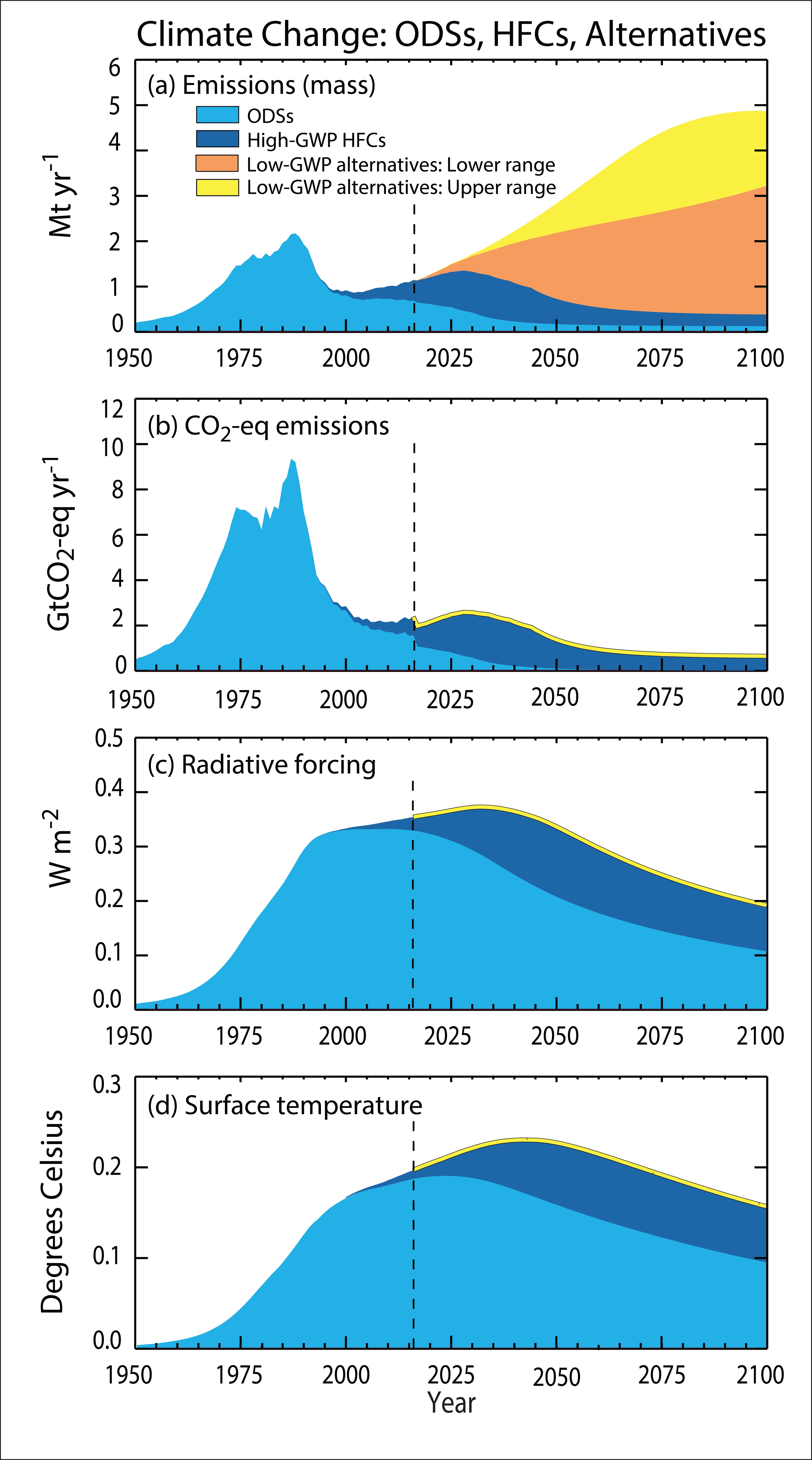
Historical and projected contributions to climate change from emissions of ODSs, high-GWP HFCs, and low-GWP alternatives have been calculated, assuming full compliance with the Montreal Protocol, including the Kigali Amendment (Figure ES-5).
Future CO2-eq emissions of HFCs from 2020 to 2060 under the Kigali Amendment are about half of those in a scenario without any HFC controls. Assuming compliance, projected cumulative emissions of HFCs from 2020 to 2060 decrease to approximately 60 GtCO2-eq. CFCs from known banks and HCFCs cumulatively contribute approximately 3 Gt and 9 GtCO2-eq emissions, respectively, over the same time period. For comparison, cumulative CO2 emissions from fossil fuel usage are projected over this time period to be 760 GtCO2 in the RCP-2.6 scenario and 1700 GtCO2 in the RCP-6.0 scenario. The peak in annual CO2-eq emissions of all HFCs together is expected to be much smaller than the peak in ODS emissions (Figure ES-5).
A faster phasedown of HFCs than required by the Kigali Amendment would further limit climate change from HFCs. One way to achieve this phasedown would be more extensive replacement of high-GWP HFCs with commercially available low-GWP alternatives in refrigeration and air-conditioning equipment. Figure ES-9 shows the impact of a complete elimination of production of HFCs starting in 2020, and their substitution with low-GWP HFCs, which would avoid an estimated cumulative 53 GtCO2‑eq emission during 2020–2060.
Improvements in energy efficiency in refrigeration and air-conditioner equipment during the transition to low-GWP alternative refrigerants can potentially double the climate benefits of the HFC phasedown of the Kigali Amendment.
Total radiative forcing from the controlled ODSs and their replacements continues to be strongly limited by the Montreal Protocol, including the Kigali Amendment. The radiative forcing from CFCs has been declining since the early 2000s. The sum of CFC and HCFC radiative forcing has been stable for about two decades and is just starting to decline. The total forcing from CFC and HCFCs and their HFC replacements is projected to continue to increase gradually for the next decade or two. After that, the ODS and HFC restrictions of the Montreal Protocol, if adhered to, ensure a continued decline in total RF from ODSs and their replacements through the rest of the century.
Global warming potentials, global temperature potentials, and ozone depletion potentials of hundreds of HCFCs have been calculated and are presented, most for the first time in an assessment. These data include all the HCFCs listed under Annex C, Group I of the Montreal Protocol, many of which did not have estimated GWPs at the time of the adoption of the Kigali Amendment. This information is significant since the Kigali Amendment uses CO2-eq production and consumption of HFCs and HCFCs as a metric for the baseline determination of the HFC phasedown.
Impacts of climate change and other processes on future stratospheric ozone
Anthropogenic activity associated with climate change could have potentially important impacts on the future of the ozone layer.
The wide range of possible future levels of CO2, CH4, and N2O represents an important limitation to making accurate projections of the ozone layer [see Ozone recovery and ozone-climate interactions section]. future ODS atmospheric concentrations are highly constrained by the Montreal Protocol, the range in projected ozone levels across the ODS scenarios is much smaller than that associated with GHG changes.
Intentional long-term geoengineering applications that substantially increase stratospheric aerosols to mitigate global warming by reflecting sunlight would alter the stratospheric ozone layer. The estimated magnitude and even the sign of ozone changes in some regions are uncertain because of the high sensitivity to variables such as the amount, altitude, geographic location, type of injection and the halogen loading. An increase of the stratospheric sulfate aerosol burden in amounts sufficient to substantially reduce global radiative forcing would delay the recovery of the Antarctic ozone hole. Much less is known about the effects on ozone from geoengineering solutions using non-sulfate aerosols.
Scientific Summaries of the Chapters
Chapter 1: Update on Ozone-Depleting Substances (ODSs) and other Gases of Interest to the Montreal Protocol
This chapter concerns atmospheric changes in ozone-depleting substances (ODSs), such as chlorofluorocarbons (CFCs), halons, chlorinated solvents (e.g., CCl4 and CH3CCl3) and hydrochlorofluorocarbons (HCFCs), which are controlled under the Montreal Protocol. Furthermore, the chapter updates information about ODSs not controlled under the Protocol, such as methyl chloride (CH3Cl) and very short-lived substances (VSLSs). In addition to depleting stratospheric ozone, many ODSs are potent greenhouse gases.
Mole fractions of ODSs and other species are primarily measured close to the surface by global or regional monitoring networks. The surface data can be used to approximate a mole fraction representative of the global or hemispheric tropospheric abundance. Changes in the tropospheric abundance of an ODS result from a difference between the rate of emissions into the atmosphere and the rate of removal from it. For gases that are primarily anthropogenic in origin, the difference between northern and southern hemispheric mole fractions is related to the global emission rate because these sources are concentrated in the northern hemisphere.
The abundances of the majority of ODSs that were originally controlled under the Montreal Protocol are now declining, as their emissions are smaller than the rate at which they are destroyed. In contrast, the abundances of most of the replacement compounds, HCFCs and hydrofluorocarbons (HFCs, which are discussed in Chapter 2), are increasing.
Tropospheric chlorine
Total tropospheric chlorine is a metric used to quantify the combined globally averaged abundance of chlorine in the troposphere due to the major chlorine-containing ODSs. The contribution of each ODS to total tropospheric chlorine is the product of its global tropospheric mean mole fraction and the number of chlorine atoms it contains.
-
Total tropospheric chlorine (Cl) from ODSs continued to decrease between 2012 and 2016. Total tropospheric chlorine in 20166 was 3,287 ppt (where ppt refers to parts per trillion as a dry air mole fraction), 11% lower than its peak value in 1993, and about 0.5% lower than reported for 2012 in the previous Assessment. Of the 2016 total, CFCs accounted for about 60%, CH3Cl accounted for about 17%, CCl4 accounted for about 10%, and HCFCs accounted for about 9.5%. The contribution from CH3CCl3 has now decreased to 0.2%. Very short-lived source gases (VSL SGs), as measured in the lower troposphere, contributed approximately 3%.
-
During the period 2012–2016, the observed rate of decline in tropospheric Cl due to controlled substances was 12.7 ± 0.97 ppt Cl yr−1, similar to the 2008–2012 period (12.6 ± 0.3 ppt Cl yr−1). This rate of decrease was close to the projections from the A1 scenario8 in the previous Assessment. However, the net rate of change was the result of a slower than projected decrease in CFCs and a slower HCFC increase than in the A1 scenario, which assumed that HCFC production from Article 5 countries would follow the maximum amount allowed under the Montreal Protocol.
-
When substances not controlled under the Montreal Protocol are also included, the overall decrease in tropospheric chlorine was 4.4 ± 4.1 ppt Cl yr−1 during 2012–2016. This is smaller than the rate of decline during the 2008–2012 period (11.8 ± 6.9 ppt Cl yr−1) and smaller than the rate of decline in controlled substances because VSLS, predominantly anthropogenic dichloromethane (CH2Cl2), and methyl chloride (CH3Cl), which is mostly from natural sources, increased during this period.
-
Starting around 2013, the rate at which the CFC-11 mole fraction was declining in the atmosphere slowed unexpectedly, and the interhemispheric difference in its mole fraction increased. These changes are very likely due to an increase in emissions, at least part of which originate from eastern Asia. Assuming no change in atmospheric circulation, an increase in global emissions of approximately 10 Gg yr−1 (~15%) is required for 2014–2016, compared to 2002–2012, to account for the observed trend and interhemispheric difference. The rate of change and magnitude of this increase is unlikely to be explained by increasing emissions from banks. Therefore, these findings may indicate new production not reported to the United Nations Environment Programme (UN Environment). If the new emissions are associated with uses that substantially increase the size of the CFC-11 bank, further emissions resulting from this new production would be expected in future.
Compared to 2008–2012, for the period 2012–2016, mole fractions of CFC-1149 declined more slowly, CFC-13 continued to rise, and CFC-115 exhibited positive growth after previously showing near-zero change. These findings likely indicate an increase or stabilization of the emissions of these relatively low abundance compounds, which is not expected given their phaseout for emissive uses under the Montreal Protocol. For CFC-114 and -115, regional analyses show that some of these emissions originate from China. There is evidence that a small fraction of the global emissions of CFC-114 and -115 are due to their presence as impurities in some HFCs. However, the primary processes responsible are unknown.
The rate at which carbon tetrachloride (CCl4) has declined in the atmosphere remains slower than expected from its reported use as a feedstock. This indicates ongoing emissions of around 35 Gg yr−1. Since the previous Assessment, the best estimate of the global atmospheric lifetime of CCl4 has increased from 26 to 32 years, due to an upward revision of its lifetime with respect to loss to the ocean and soils. New sources have been proposed including significant by-product emissions from the production of chloromethanes and perchloroethylene and from chlor-alkali plants. With these changes in understanding, the gap between top-down and bottom-up emissions estimates has reduced to around 10 Gg yr−1, compared to 50 Gg yr−1 previously.
Combined emissions of the major HCFCs have declined since the previous Assessment. Emissions of HCFC-22 have remained relatively stable since 2012, while emissions of HCFC-141b and -142b declined between 2012 and 2016, by around 10% and 18%, respectively. These findings are consistent with a sharp drop in reported HCFC consumption after 2012, particularly from Article 5 countries.
Emissions of the compounds HCFC-133a and HCFC-31, for which no current intentional use is known, have been detected from atmospheric measurements. Research to date suggests that these gases are unintentional by-products of HFC-32, HFC-134a, and HFC-125 production.
Tropospheric bromine
Total tropospheric bromine is defined in analogy to total tropospheric chlorine. Even though the abundance of bromine is much smaller than that of chlorine, it has a significant impact on stratospheric ozone because it is around 60–65 times more efficient than chlorine as an ozone-destroying catalyst.
Total tropospheric bromine from controlled ODSs (halons and methyl bromide) continued to decrease and by 2016 was 14.6 ppt, 2.3 ppt below the peak levels observed in 1998. In the 4-year period prior to the last Assessment, this decrease was primarily driven by a decline in methyl bromide (CH3Br) abundance, with a smaller contribution from a decrease in halons. These relative contributions to the overall trend have now reversed, with halons being the main driver of the decrease of 0.15 ± 0.04 ppt Br yr−1 between 2012 and 2016.
The mole fractions of halon-1211, halon-2402, and halon-1202 continued to decline between 2012 and 2016. Mole fractions of halon-1301 increased during this period, although its growth rate dropped to a level indistinguishable from zero in 2016. Emissions of halon-2402, halon-1301, and halon-1211, as derived from atmospheric observations, declined or remained stable between 2012 and 2016.
Methyl bromide (CH3Br) mole fractions continued to decline between 2012 and 2015 but showed a small increase (2–3%) between 2015 and 2016. This overall reduction is qualitatively consistent with the controls under the Montreal Protocol. The 2016 level was 6.8 ppt, a reduction of 2.4 ppt from peak levels measured between 1996 and 1998. The increase between 2015 and 2016 was the first observation of a positive global change for around a decade or more. The cause of this increase is yet to be explained. However, as it was not accompanied by an increased interhemispheric difference, it is unlikely that this is related to anthropogenic emissions in the Northern Hemisphere. By 2016, controlled CH3Br consumption dropped to less than 2% of the peak value, and total reported fumigation emissions have declined by more than 85% since their peak in 1997. Reported consumption in quarantine and pre-shipment (QPS) uses of CH3Br, which are not controlled under the Montreal Protocol, have not changed substantially over the last two decades.
Halogenated very short-lived substances (VSLSs)
VSLSs are defined as trace gases whose local lifetimes are shorter than 0.5 years and have nonuniform tropospheric abundances. These local lifetimes typically vary substantially over time and space. Of the very short-lived source gases (VSL SGs) identified in the atmosphere, brominated and iodinated species are predominantly of oceanic origin, while chlorinated species have significant additional anthropogenic sources. VSLSs will release the halogen they contain almost immediately once they enter the stratosphere and will thus play an important role in the lower stratosphere in particular. Due to their short lifetimes and their atmospheric variability the quantification of their contribution is much more difficult and has much larger uncertainties than for long-lived compounds.
Total tropospheric chlorine from VSL SGs in the background lower atmosphere is dominated by anthropogenic sources. It continued to increase between 2012 and 2016, but its contribution to total chlorine remains small. Global mean chlorine from VSLSs in the troposphere has increased from about 90 ppt in 2012 to about 110 ppt in 2016. The relative VSLS contribution to stratospheric chlorine input derived from observations in the tropical tropopause layer has increased slightly from 3% in 2012 to 3.5% in 2016.
Dichloromethane (CH2Cl2), a VSL SG that has predominantly anthropogenic sources, accounted for the majority of the change in total chlorine from VSLSs between 2012 and 2016 and is the main source of VSLS chlorine. The global mean abundance reached approximately 35–40 ppt in 2016, which is about a doubling compared to the early part of the century. The increase slowed substantially between 2014 and 2016. Emissions from southern and eastern Asia have been detected for CH2Cl2.
There is further evidence that VSLSs contribute ~5 (3–7) ppt to stratospheric bromine, which was about 25% of total stratospheric bromine in 2016. The main sources for brominated VSLSs are natural, and no long-term change is observed. While the best estimate of 5 ppt has remained unchanged from the last Assessment, the assessed uncertainty range has been reduced. Due to the decline in the abundance of regulated bromine compounds, the relative contribution of VSLSs to total stratospheric bromine continues to increase.
Stratospheric chlorine and bromine
In the stratosphere, chlorine and bromine can be released from organic source gases to form inorganic species, which participate in ozone depletion. In addition to estimates of the stratospheric input derived from the tropospheric observations, measurements of inorganic halogen loading in the stratosphere are used to determine trends of stratospheric chlorine and bromine.
Hydrogen chloride (HCl) is the major reservoir of inorganic chlorine (Cly) in the mid to upper stratosphere. Satellite-derived measurements of HCl (60°N–60°S) in the middle stratosphere show a long-term decrease of HCl at a rate of around 0.5% yr−1, in good agreement with expectations from the decline in tropospheric chlorine. In the lower stratosphere, a decrease was observed over the period from 1997 to 2016, while significant differences in the trends are seen over the period 2005 to 2016 between various datasets and altitude/geographical regions. A similar behavior is observed for total column measurements, likely reflecting variability in stratospheric dynamics and chemistry. Total chlorine input to the stratosphere of 3,290 ppt is derived for 2016 from measurements of long-lived ODSs at the surface and VSLSs in the upper troposphere. About 80% of this input is from substances controlled under the Montreal Protocol.
Total stratospheric bromine, derived from observations of bromine monoxide (BrO), continued to decrease at a rate of about 0.75% yr−1 from 2004 to 2014. This decline is consistent with the decrease in total tropospheric organic bromine, based on measurements of CH3Br and the halons. A total bromine input to the stratosphere of 19.6 ppt is derived for 2016, combined from 14.6 ppt of long-lived gases and 5 ppt from VSLSs not controlled under the Montreal Protocol. Anthropogenic emissions of all brominated long-lived gases are controlled, but as CH3Br also has natural sources, more than 50% of the bromine reaching the stratosphere is now estimated to be from sources not controlled under the Montreal Protocol. There is no indication of a long-term change in natural sources to stratospheric bromine.
Equivalent effective stratospheric chlorine (EESC)
EESC is the chlorine-equivalent sum of chlorine and bromine derived from ODS tropospheric abundances, weighted to reflect their expected depletion of stratospheric ozone. The growth and decline in EESC depends on a given tropospheric abundance propagating to the stratosphere with varying time lags (on the order of years) associated with transport. Therefore, the EESC abundance, its peak timing, and its rate of decline are different in different regions of the stratosphere. Recent suggestions of a refinement in the calculation method for EESC result in somewhat lower estimates on how far the stratospheric reactive halogen loading has recovered.
By 2016, EESC had declined from peak values by about 9% for polar winter conditions and by about 13–17% for mid-latitude conditions. This drop is 31–43% of the decrease required for EESC in mid-latitudes to return to the 1980 benchmark level, and about 18–19% of the decrease required for EESC in polar regions to return to the 1980 benchmark level10. The rate at which EESC is decreasing has slowed, in accordance with a slowdown of the decrease in tropospheric chlorine. The ranges given reflect the different methods for calculating EESC. Differences in halogen recovery levels from previous Assessments are also due to differences in assumed fractional release factors.
Tropospheric and stratospheric fluorine
While fluorine has no direct impact on stratospheric ozone, many fluorinated gases are strong greenhouse gases, and their emission is often related to the replacement of chlorinated substances regulated under the Montreal Protocol. For this reason, trends in fluorine are also assessed in this report.
The main sources of fluorine in the troposphere and in the stratosphere are CFCs, HCFCs, and HFCs. In contrast to total chlorine, total fluorine in the troposphere continued to increase between 2012 and 2016, at a rate of 1.7% yr−1. This increase shows the decoupling of the temporal trends in fluorine and chlorine due to the increasing emissions of HFCs (see Chapter 2). The total atmospheric-column abundance of inorganic fluorine, which is mainly stratospheric, has continued to increase at a rate of about 1% yr−1 over the period 2007–2016.
Effect of ozone-depleting substances (ODSs) on climate
The total direct radiative forcing11 of CFCs continues to be much higher than that of HCFCs. However, radiative forcing from CFCs has dropped by about 7% since its peak in 2000 to about 250 mW m−2 in 2016 (approximately 13% that of CO2), while radiative forcing from HCFCs increased to 58 mW m−2 in 2016 (approximately 3% that of CO2). The total direct radiative forcing due to CFCs, HCFCs, halons, CCl4 and CH3CCl3 was 327 mW m–2 in 2016 (approximately 16% that of CO2).
CO2-equivalent emissions12 of CFCs and HCFCs were approximately equal in 2016. The CO2-equivalent emission from the sum of all CFCs or the sum of all HCFCs was approximately 0.8 Gt in 2016. The CO2-equivalent emission from the sum of CFCs, HCFCs, halons, CCl4 and CH3CCl3 was approximately 1.7 Gt in 2016.
Other gases that affect ozone and climate
Mole fractions of many other gases that affect both ozone and climate have changed since the previous Assessment. The atmospheric abundance of methane has continued to increase following a period of stagnation in the early 2000s. The drivers of the changing trend are disputed. Nitrous oxide continues to grow relatively steadily in the atmosphere. The global mole fractions of the fluorinated species sulfur hexafluoride (SF6), nitrogen trifluoride (NF3), sulfuryl fluoride (SO2F2), and the perfluorocarbons (PFCs such as CF4 and C2F6) have continued to grow. In contrast, the abundance of the sulfur-containing compounds sulfur dioxide (SO2) and carbonyl sulfide (COS) has not changed substantially.
Chapter 2: Hydrofluorocarbons (HFCs)
The Montreal Protocol is an international agreement designed to heal the ozone layer. It outlines schedules for the phase-out of ozone-depleting substances (ODSs) such as chlorofluorocarbons (CFCs), hydrochlorofluorocarbons (HCFCs), chlorinated solvents, halons, and methyl bromide. As a result of this phase-out, alternative chemicals and procedures were developed by industry for use in many applications including refrigeration, air-conditioning, foam-blowing, electronics, medicine, agriculture, and fire protection. Hydrofluorocarbons (HFCs) were used as ODS alternatives in many of these applications because they were suitable substitutes and they do not contain ozone-depleting chlorine or bromine; in addition, most HFCs have smaller climate impacts per molecule than the most widely used ODSs they replaced. Long-lived HFCs, CFCs, and HCFCs, however, are all potent greenhouse gases, and concerns were raised that uncontrolled future use of HFCs would lead to substantial climate warming.
As a result of these concerns, HFCs were included as one group of greenhouse gases for which emissions controls were adopted by the 1997 Kyoto Protocol under the 1992 United Nations Framework Convention on Climate Change (UNFCCC). Consequently, developed countries (those listed in Annex I to this Convention, or “Annex I” Parties) supply annual emission estimates of HFCs to the UNFCCC.
Since the Kyoto Protocol only specified limits on the sum of all controlled greenhouse gases, emissions of HFCs were not explicitly controlled. However, following the Kyoto Protocol, some countries enacted additional controls specifically limiting HFC use based on their global warming potentials (GWPs). Ultimately the Kigali Amendment to the Montreal Protocol was agreed upon in 2016, and this Amendment supplies schedules for limiting the production and consumption of specific HFCs. Although the radiative forcing supplied by HFCs is currently small, this Amendment was designed to ensure that the radiative forcing from HFCs will not grow uncontrollably in the future. The Kigali Amendment will come into force at the start of 2019. HFC concentrations are currently monitored through atmospheric measurements. All HFCs with large abundances are monitored, as are most with small abundances.
Most HFCs that are emitted to the atmosphere are intentionally produced for use in a variety of applications that were once dependent on ODSs. An exception is HFC-23, which is emitted to the atmosphere primarily as a by-product of HCFC-22 production. HFC-23 is also unique in that it has a substantially longer atmospheric lifetime and higher GWP than nearly all other HFCs. As a result, the Kigali Amendment includes different control schedules for HFC-23 production than for other HFCs. To date, HFC-23 emissions have been partially abated in developed countries through regulations or voluntary measures and in developing countries with assistance from the UNFCCC’s Clean Development Mechanism (CDM).
-
Atmospheric mole fractions of most currently measured HFCs are increasing in the global atmosphere at accelerating rates, consistent with expectations based on the ongoing transition away from use of ozone-depleting substances.
-
HFC-134a remained the most abundant HFC in the atmosphere, reaching a global mean surface mole fraction of nearly 90 ppt in 2016. Its rate of increase averaged 5.6 ± 0.2 ppt yr−1 (7.3 ± 0.2 % yr−1) during 2012–2016, which is about 0.6 ppt yr−1 faster than the mean increase for 2008–2012.
-
The next four most abundant HFCs in 2016 were HFC-23, HFC-125, HFC-143a, and HFC-32. Their global mean surface mole fractions in 2016 were 28.9 ppt, 20.4 ppt, 19.2 ppt, and 11.9 ppt, respectively. Mole fractions of these HFCs increased during 2012–2016 by an average of 1.0 ppt yr−1 for HFC-23, 2.1 ppt yr−1 for HFC-125, 1.5 ppt yr−1 for HFC-143a, and 1.6 ppt yr−1 for HFC-32; for all of these gases, these rates are faster than the average growth rates reported for 2008–2012 in the last Assessment.
-
Global mole fractions of most HFCs increased through 2016 at rates similar to those projected in the baseline scenario of the last Assessment, despite the fact that this scenario was created nearly a decade ago. The HFCs for which mole fractions are increasing substantially less rapidly than originally projected include HFC-152a, HFC-365mfc, and HFC-245fa.
-
Radiative forcing from measured HFCs continues to increase; it currently amounts to 1% of the total forcing from all long-lived greenhouse gases. The radiative forcing arising from measured atmospheric mole fractions of HFCs totaled 0.030 W m−2 in 2016, up by 36% from 0.022 W m−2 in 2012; HFC-134a accounted for 47% of this forcing in 2016, while the next largest contributors were HFC-23 (17%), HFC-125 (15%) and HFC-143a (10%). Total HFC radiative forcing in 2016 accounted for ~10% of the 0.33 W m−2 supplied by ODSs (see Chapter 1), and 1.0% of the 3 W m−2 supplied by all long-lived GHGs combined, including CO2, CH4, N2O, ODSs and HFCs.
Global emissions of nearly all measured HFCs continue to increase; they currently amount to ~1.5% of total emissions from all long-lived greenhouse gases (CO2, CH4, N2O, and long-lived halocarbons) in CO2-equivalent emissions. As derived from atmospheric observations, total emissions of HFCs increased by 23% from 2012 to 2016 and summed to 0.88 (± 0.07) GtCO2-eq yr−1 in 2016; this increase outpaced decreases in CO2-eq emissions from CFCs and HCFCs. These CO2-eq HFC emissions stem primarily from four gases: HFC-134a (34% of total), HFC-125 (24% of total), HFC-23 (18% of total), and HFC-143a (16% of total). HFC CO2-eq emissions were comparable to those of CFCs (0.8 ± 0.3 GtCO2-eq yr−1) and HCFCs (0.76 ± 0.11 GtCO2-eq yr−1) in 2016.
HFC emissions estimated from the combination of inventory reporting and atmospheric observations indicate that the HFC emissions originate from both developed and developing countries. Large differences are observed between global total emissions derived from atmospheric observations and the totals reported to the UNFCCC. These differences arise primarily because only developed (Annex I) countries are obligated to report HFC emissions to the UNFCCC. When summed, these reported HFC emissions account for less than half of the global total inferred from observations (as CO2-eq emissions).
Annual global emissions of HFC-23 derived from atmospheric measurements have varied substantially in recent years. This variability is mostly consistent with expectations based on reported HCFC-22 production and reported and estimated HFC-23 emissions. This long-lived HFC is emitted to the atmosphere primarily as a by-product of HCFC-22 production. HFC-23 emissions, after reaching a low of ~10 Gg yr−1 (0.13 GtCO2‑eq yr−1) 2009–2010, owing in part to destruction in developing countries facilitated under the UNFCCC’s Clean Development Mechanism (CDM), increased and subsequently peaked at ~14 Gg yr−1 (0.18 GtCO2-eq yr−1) in 2013–2014. The mean global emission rate over 2013–2014 is slightly higher than that derived for 2005–2006, when CDM-facilitated destruction had yet to be fully implemented. Global emissions estimated from observations for 2015 and 2016 dropped below the 2013–2014 peak; emissions in 2016 were 12.3 ± 0.7 Gg yr−1 (0.16 GtCO2-eq yr−1), or approximately 2 Gg yr−1 below those in 2014. New controls put in place under the Kigali Amendment mandate HFC-23 by-product destruction, to the extent practicable, beginning in 2020. These controls are expected to limit future emissions and thus slow or reverse atmospheric concentration increases of this potent greenhouse gas.
Some next-generation substitute chemicals with very low GWPs (unsaturated HCFCs and unsaturated HFCs, also known as hydrofluoroolefins, or HFOs) have now been detected in ambient air, consistent with the transition to these compounds being underway. Unsaturated HFCs and HCFCs are replacement compounds for some long-lived HCFCs and HFCs. Because unsaturated HFCs have short atmospheric lifetimes (days) and GWPs typically less than 1 they are not included as controlled substances in the Kigali Amendment to the Montreal Protocol. Very low mole fractions (typically below 1 ppt) of two unsaturated HFCs (HFC-1234yf and HFC-1234ze(E)) have been measured at a continental background European site.
Global adherence to the HFC phasedown schedule of the 2016 Kigali Amendment to the Montreal Protocol would substantially reduce future projected global HFC emissions. Emissions are projected to peak before 2040 and decline to less than 1 GtCO2-eq yr−1 by 2100. Only marginal increases are projected for CO2-eq emissions of the low-GWP alternatives despite substantial projected increases in their emission mass. The estimated avoided HFC emissions as a result of this Amendment is 2.8–4.1 GtCO2-eq yr−1 emissions by 2050 and 5.6–8.7 GtCO2-eq yr−1 by 2100. For comparison, total CH4 emissions in 2100 are projected to be 7.0 and 25 GtCO2-eq yr−1 in the RCP-6.0 and RCP-8.5 scenarios, respectively, and total N2O emissions in 2100 are projected to be 5.0 and 7.0 GtCO2-eq yr−1 in these same scenarios.
The 2016 Kigali Amendment to the Montreal Protocol, assuming global compliance, is expected to reduce future radiative forcing due to HFCs by about 50% in 2050 compared to the forcing from HFCs in the baseline scenario. Currently (in 2016), HFCs account for a forcing of 0.025 W m−2 not including 0.005 from HFC-23; forcing from these HFCs was projected to increase up to 0.25 W m−2 by 2050 (excluding a contribution from HFC-23) with projected increased use and emissions in the absence of controls. With the adoption of the Kigali Amendment, a phasedown schedule has been agreed for HFC production and consumption in developed and developing countries under the Montreal Protocol. With global adherence to this Amendment in combination with national and regional regulations that were already in place in, e.g., Europe, the USA, and Japan, along with additional recent controls in other countries, future radiative forcing from HFCs is projected to reach 0.13 W m−2 by 2050 (excluding HFC-23), or about half the forcing projected in the absence of these controls.
The Kigali Amendment and national and regional regulations are projected to reduce global average warming in 2100 due to HFCs from 0.3–0.5°C in a baseline scenario to less than 0.1°C. If the global production of HFCs were to cease in 2020, the surface temperature contribution of HFC emissions would stay below 0.02°C for the whole 21st century. The magnitude of the avoided temperature increase due to the provisions of the Kigali Amendment is substantial in the context of the 2015 UNFCCC Paris Agreement, which aims to limit global temperature rise to well below 2.0°C above pre-industrial levels and to pursue further efforts to limit the temperature increase to 1.5°C.
Improvements in energy efficiency in refrigeration and air-conditioning equipment during the transition to low-GWP alternative refrigerants can potentially double the climate benefits of the HFC phasedown of the Kigali Amendment. The conversion from equipment using HFC refrigerants with high GWPs to refrigerants with lower GWPs, which will most likely result from the Kigali Amendment, provides an opportunity to consider other technological improvements that offer additional climate benefits. The total climate impact related to refrigerant use and associated emissions is not only associated with the radiative properties and lifetime of the refrigerant, but also with CO2 emissions resulting from the energy used by the equipment over its entire life cycle. The use of a refrigerant with a lower GWP than the currently-used HFCs (i.e., following the Kigali Amendment) offers the opportunity to redesign equipment and improve its energy efficiency. For example, a 30% improvement in the energy efficiency of the global stock of mini-split air conditioners (the most widely used air conditioning systems today) in 2030 would provide a climate benefit comparable to replacing the mix of current HFC refrigerants commonly used in this application (which have GWPs averaging about 2,000) with a mix of alternatives that have GWPs of less than about 5 to about 700. An energy efficiency improvement of 30% is estimated to be technically and economically feasible and cost-effective in many economies.
Some HFCs degrade in the environment to produce trifluoroacetic acid (TFA), a persistent toxic chemical. The environmental effects of this source of TFA are currently small and are expected to remain negligible over the next decades. Atmospheric degradation of HFC-1234yf, a replacement compound for some long-lived HCFCs and HFCs, produces TFA. Potential impacts beyond a few decades of this TFA source could require future evaluation due to the environmental persistence of TFA and uncertainty in future emissions of HFC-1234yf and other HFCs that produce TFA upon degradation.
Improvements in the understanding of reaction rates have been incorporated into revised lifetime estimates for saturated and unsaturated HFCs. Most of these changes are small, although lifetimes of HFC-245cb (CF3CF2CH3), octafluorocyclopentene (cyclo-CF=C4F7-), (E)-HFO-1214yc ((E)-CF3CH=CHCF3), and (E)-HFO-1438mzz ((E)-CF3CH=CHC2F5) were noticeably changed because the relevant reaction rate information has become available for the first time. Lifetimes for a few HFCs considered here remain estimates based on either analogy with similar compounds or structure–activity relationships.
Chapter 3: Update on Global Ozone: Past, Present, and Future
This chapter deals with the evolution of global ozone outside of the polar regions. The increase of ozone-depleting substance (ODS) concentrations caused the large ozone decline observed from the early satellite era (circa 1980) to the mid-1990s. Since the late 1990s, concentrations of ODSs have been declining due to the successful implementation of the Montreal Protocol. Ozone concentrations show latitudinally dependent increases in the upper stratosphere for the 2000–2016 period; changes in other parts of the stratosphere are not yet statistically significant. A new suite of model simulations confirms previous results for the upper stratosphere that about half of the observed increase is associated with declining ODSs. Ozone column trends are likewise positive but not generally statistically significant. Their overall evolution is, however, compatible with the decline in equivalent effective stratospheric chlorine (EESC).
Over the next decades, we expect increasing global mean stratospheric ozone columns, as ODSs continue to decline. Emissions of greenhouse gases (GHGs), especially carbon dioxide (CO2), methane (CH4), and nitrous oxide (N2O), will also affect the evolution of global stratospheric ozone, particularly in the second half of the 21st century, when ODS concentrations are expected to be low.
Past changes in total column ozone
-
Ground- and space-based observations indicate that there is no statistically significant trend in near-global (60°S–60°N) column ozone over the 1997–2016 period. These datasets show an increase of between 0.3% and 1.2% decade−1 since 1997, with uncertainties of about 1% decade−1. These findings are consistent with our understanding of the processes that control ozone.
In middle and high latitudes, the increase in total column ozone expected to arise from the 15% decline in EESC since 1997 is small (~1% decade−1) relative to the large, dynamically forced year-to-year variations of ~5%.
In the tropics, where halogen-driven ozone loss is small in the lower stratosphere, total column ozone has not varied significantly with ODS concentrations, except under conditions of high volcanic aerosol loading (e.g., from the eruption of Mt. Pinatubo in 1991).
-
Outside the tropics, present-day (2014–2017) total ozone columns from ground-based and space-based observations remain lower than 1964–1980 column ozone by
about 2.2% for the near-global average (60°S–60°N)
about 3.0% in the Northern Hemisphere mid-latitudes (35°N–60°N)
about 5.5% in the Southern Hemisphere mid-latitudes (35°S–60°S)
These values are essentially the same as in the last Assessment, given uncertainties associated with natural variability and instrumental accuracy. The larger depletion in the Southern Hemisphere is linked to the Antarctic ozone hole.
Past changes in ozone profiles
Additional and improved datasets and focused studies evaluating trend uncertainties have strengthened our ability to assess ozone profile changes. Analysis of data from the upper stratosphere shows increases that are consistent with those suggested in the last Assessment. There is some evidence for a dynamically driven decrease in ozone in the lower stratosphere from 2000 to 2016, but robust trends have not been identified for this region. New chemistry–climate model (CCM) simulations that include realistic time variations of GHG and ODS concentrations are analyzed using the same trend model as for the observations; this allows attribution of changes in ozone to different processes.
Measurements show increases of ozone in the upper stratosphere over the period 2000-2016. Following a large decline of 5 to 7% decade−1 through the 1980s and middle 1990s, upper stratospheric ozone has increased by 1 to 3% decade−1 since 2000. The largest confidence is in northern mid-latitudes, where the positive trend is statistically significant between 35- and 45-km altitude. Confidence in trends in the tropics and southern mid-latitudes is not as high due to larger discrepancies between trends from individual measurement records.
Model simulations attribute about half of the observed upper stratospheric ozone increase after 2000 to the decline of ODSs since the late 1990s. The other half of the ozone increase is attributed to the slowing of gas-phase ozone destruction cycles, which results from cooling of the upper stratosphere caused by increasing GHGs.
There is some evidence for a decrease in lower stratospheric ozone from 2000 to 2016. This decrease is most consistent across datasets in the tropics, but is not statistically significant in most analyses. Much of the apparent decline was reversed by an abrupt increase in ozone in 2017, indicating that longer records are needed to robustly identify trends in this region. Model simulations attribute the variations in lower stratospheric ozone over this period primarily to dynamical variability.
Assessing the consistency between stratospheric profile trends and total column ozone trends requires changes in tropospheric ozone to be well quantified. A recent assessment of tropospheric column ozone trends, however, shows large disagreements in the sign and magnitude of the observed trends over the past decade and a half.
Future ozone changes
The baseline climate change scenario used in the new model simulations differs from the previous Assessment, because new emissions scenarios were used. The key drivers of future ozone levels continue to be declining ODS concentrations, upper stratospheric cooling because of increased GHGs, and the possible strengthening of the Brewer-Dobson circulation from climate change. The new emissions scenarios lead to slight differences in the relative contributions of these processes in various latitude and altitude regions and a delay in return dates for ozone compared to the previous Assessment.
-
Estimated dates of return of total column ozone to 1980 values are generally a few years later than given in the previous Assessment and vary considerably between scenarios. For the baseline scenario (RCP-6.0), they are:
around mid-century for near-global mean annually averaged ozone;
most likely before the middle of the century (~2035) for annually averaged Northern Hemisphere mid-latitude ozone;
around mid-century for annually averaged Southern Hemisphere mid-latitude ozone.
CO2, CH4, and N2O will be the main drivers of 60°S–60°N stratospheric ozone changes in the second half of the 21st century. These gases impact both chemical cycles and the stratospheric overturning circulation, with a larger response in stratospheric ozone associated with stronger climate forcing. By 2100, the stratospheric column is expected to decrease in the tropics by about 5 DU for RCP-4.5 and about 10 DU for RCP-8.5 relative to 1980 values, with the net total column change projected to be smaller (about 5 DU) because of offsetting increases in tropospheric ozone.
Given that ODS levels are expected to decline slowly in coming years, a large enhancement of stratospheric sulfate aerosol in the next decades would result in additional chemical ozone losses. Possible sources of additional stratospheric sulfate aerosol include volcanic eruptions (like Mt. Pinatubo in 1991) and geoengineering. Even when ODS levels have declined substantially, a large injection of volcanic halogens into the stratosphere could drive substantial ozone losses in the presence of aerosol surfaces.
Future ozone recovery and the projected strengthening of the Brewer-Dobson circulation (BDC) are likely to lead to increases in the stratosphere-to-troposphere (STT) flux of ozone via increases in mid-latitude lower stratospheric ozone and mass flux. The net impact of increased STT flux on the tropospheric ozone burden is highly model and scenario dependent. Most studies suggest it will be small relative to other factors, such as concurrent changes in precursor emissions, temperature, and water vapor.
Chapter 4: Update on Polar Ozone: Past, Present, and Future
The chemical and dynamical processes controlling polar ozone are well understood. Polar ozone depletion is fundamentally driven by anthropogenic chlorine and bromine, with the severity of the chemical loss each year in both hemispheres strongly modulated by meteorological conditions (temperatures and winds), and, to a lesser extent, by the stratospheric aerosol loading and the solar cycle. As noted in prior Assessments, the stratospheric halogen concentration resulting from the emission of ozone-depleting substances (ODSs) reached its peak in the polar regions around the turn of the century and has been gradually declining since then in response to actions taken under the Montreal Protocol and its Amendments and adjustments. Early signs of ozone recovery are now beginning to appear in the Antarctic; as the observational record lengthens, clearer ozone hole recovery trends are expected to emerge against the background of natural variability. Nevertheless, the Antarctic ozone hole will continue to be a recurring phenomenon until the middle of the century. The Arctic is more dynamically variable, precluding identification of a significant increase in Arctic ozone, and cold conditions conducive to substantial ozone loss may still occur in a particular year in the coming decades. New chemistry–climate model (CCM) projections largely confirm previous studies that in both hemispheres, spring polar total column ozone will return to 1980 historical levels in the coming decades, albeit with a delay of a few years due to updated future ODS and greenhouse gas (GHG) emissions scenarios.
Observed changes in polar ozone
The characteristics of the October Antarctic ozone hole in the years since 2014 have generally been within the range observed since the early 1990s. In 2015, however, the ozone hole was particularly large and long-lasting, as a result of a cold and undisturbed polar stratospheric vortex. Aerosols from the Calbuco volcanic eruption in April 2015 are also believed to have contributed to the large ozone hole observed that year. Conversely, in 2017, the Antarctic ozone hole was very small due to a warm and unusually disturbed polar vortex.
Several lines of evidence have started to emerge indicating an increase in Antarctic stratospheric ozone during September. Statistically significant trends since the year 2000 have now been identified showing an increase in observed ozone and a decrease in ozone hole size and depth. Although accounting for the large degree of natural variability is challenging, the weight of evidence from statistical analyses and modeling studies suggests that the decline in ODSs made a substantial contribution to these trends.
In the Arctic, the exceptionally low ozone abundances of spring 2011 have not been observed again in the last four years. Arctic stratospheric springtime ozone is dominated by large year-to-year dynamically induced variability of the polar vortex, with severe ozone loss occurring in very cold years, such as 2011. Extreme meteorological conditions in the early 2015/2016 winter led to rapid ozone loss, but a sudden stratospheric warming (SSW) at the beginning of March 2016 curtailed the chemical processes which lead to ozone destruction about a month earlier than in 2011, keeping ozone above record low levels. Arctic ozone trends are small compared to the dynamical variability, and thus a recovery trend remains undetectable in observations over the 2000–2016 period.
Understanding of factors controlling polar ozone
Observations in the Arctic winter have demonstrated that large nitric acid trihydrate (NAT) particles are a regularly occurring phenomenon in the lower stratosphere. This knowledge improves our understanding of polar stratospheric cloud (PSC) formation and denitrification, which is important for catalytic ozone loss cycles.
Bromine-containing very short-lived substances (VSLSs) of natural origin have an important impact on the stratospheric halogen loading and consequently on stratospheric ozone loss in the polar regions. The inclusion of additional stratospheric bromine from VSLSs is necessary for models to produce a realistic simulation of polar ozone loss.
The effects of tropospheric dynamical forcing in winter on Arctic polar ozone are now better quantified. Ozone depletion in northern winters with SSWs is on average two-thirds less than in winters without SSWs, with depletion ending about one month earlier in the year. Such an SSW was a major influence on ozone levels observed in the Arctic winter of 2015/16.
Polar ozone in the middle and upper stratosphere varies by 10–15% from year to year due to energetic particle precipitation (EPP) related to solar variability. Satellite observations and model results show that NOy produced in the aurora is transported from the thermosphere down into the stratosphere in each winter, leading to stratospheric ozone decreases modulated by geomagnetic activity. The resulting variation in total column ozone is small (a few percent) but can persist for 2–3 years. Full EPP-effects were not included in current assessment models.
Model simulations show that the Montreal Protocol and its Amendments and adjustments have already brought about substantial ozone benefits. In the polar regions of both hemispheres, much larger ozone depletion than currently observed has been avoided through implementation of the Protocol.
Future evolution of polar ozone
Updated CCM projections based on full compliance with the Montreal Protocol and assuming the baseline estimate of the future evolution of GHGs (RCP-6.0) have confirmed that the Antarctic ozone hole is expected to gradually close, with springtime total column ozone returning to 1980 values shortly after mid-century (about 2060). The timing of the recovery of the ozone hole will not be significantly affected by increases in GHG concentrations. There are no substantial differences between Antarctic total ozone columns at the end of this century for the various GHG scenarios (Representative Concentration Pathways [RCPs]).
The timing of the recovery of Arctic total ozone in spring will be affected by anthropogenic climate change. Based on full compliance with the Montreal Protocol and assuming the baseline estimate of the future evolution of GHGs (RCP-6.0), Arctic springtime total ozone is expected to return to 1980 values before mid-century (2030s). New model simulations confirm that in the Arctic, enhanced GHG concentrations cause an earlier return of total column ozone to historical values than a reduction of ODSs alone.
In the second half of the 21st century CO2, CH4, and N2O will be the dominant drivers of Arctic ozone changes, assuming full compliance with the Montreal Protocol. These gases impact both chemical cycles and the stratospheric overturning circulation, with a larger response in stratospheric ozone associated with stronger climate forcing. By 2100, the stratospheric ozone column is expected to not only recover but to exceed 1960–1980 average values in the Arctic, with springtime Arctic ozone being higher by about 35 DU for RCP-4.5 and about 50 DU for RCP-8.5.
In the coming decades, substantial Arctic ozone loss will remain possible in cold winters as long as ODS concentrations are well above natural levels. Increasing GHG concentrations may cool the lower stratosphere and lead to enhanced formation of polar stratospheric clouds (PSCs) early in the Arctic winter. However, one recent study indicates that no corresponding cooling is expected in March, which is the month when persistent low temperatures lead to large chemical ozone losses.
Chapter 5: Stratospheric Ozone Changes and Climate
Since the 2014 Ozone Assessment, new research has better quantified the impact of stratospheric ozone changes on climate. Additional model and observational analyses are assessed, which examine the influence of stratospheric ozone changes on stratospheric temperatures and circulation, tropospheric circulation and composition, surface climate, the oceans, and sea ice. The new results support the main conclusions of the previous Assessment; the primary advances are summarized below.
Stratospheric temperatures
-
New estimates of satellite-observed stratospheric temperature changes show net global stratospheric cooling of around 1.5 K (at 25–35 km), 1.5 K (at 35–45 km), and 2.3 K (at 40–50 km) between 1979 and 2005, with differences between datasets of up to 0.6 K.
There are now better estimates of observed stratospheric temperature trends than were available during the last Assessment. Two datasets from satellite measurements have been re-processed and now show greater consistency in long-term temperature trends in the middle and upper stratosphere.
Satellite temperature records show smaller stratospheric cooling rates over 1998–2015 compared to 1979–1997, consistent with the observed differences in stratospheric ozone trends during these periods.
Global average temperature in the lower stratosphere (13–22 km) cooled by about 1 K between 1979 and the late 1990s but has not changed significantly since then.
-
In the lower stratosphere (13–22 km), ozone trends were the major cause of the observed cooling between the late 1970s and the mid-1990s. In the middle and upper stratosphere, however, increases in long-lived greenhouse gases played a slightly larger role than ozone changes in cooling trends over this period. Ozone recovery will continue to play an important role in future stratospheric temperature trends.
There is now improved understanding of the causes of stratospheric temperature trends and variability. For the upper stratosphere (40–50 km), new studies suggest that one-third of the observed cooling over 1979–2005 was due to ozone-depleting substances (ODSs) and associated ozone changes, while two-thirds was due to other well-mixed greenhouse gases.
Chemistry–climate models show that the magnitude of future stratospheric temperature trends is dependent on future greenhouse gas concentrations, with most greenhouse gas scenarios showing cooling in the middle and upper stratosphere over the 21st century. The projected increase in global stratospheric ozone during this period would offset part of the stratospheric cooling due to increasing greenhouse gases.
Stratospheric overturning circulation
-
There are indications that the overturning circulation in the lower stratosphere has accelerated over the past few decades.
Observations of the latitudinal profile of lower stratospheric temperature trends and changes in constituents show that tropical upwelling in the lower stratosphere has strengthened over the last ~30 years, in qualitative agreement with model simulations and reanalysis datasets.
New studies using measurements provide evidence for structural changes in the stratospheric overturning circulation which is comprised of a strengthening in the lower stratosphere and a weakening in the middle and upper stratosphere.
According to models, in addition to well-mixed greenhouse gases, changes in ODSs (and associated changes in ozone) are an important driver of past and future changes in the strength of the stratospheric overturning circulation, notably the increase in downwelling over the Antarctic over the late 20th century.
Estimates of externally forced long-term changes in the stratospheric overturning circulation from observations remain uncertain, partially due to internal variability.
Models project future increases in stratosphere–troposphere exchange of ozone as a consequence of a strengthening of the stratospheric overturning circulation and stratospheric ozone recovery.
Impacts on the troposphere, ocean, and sea ice
-
New research supports the findings of the 2014 Ozone Assessment that Antarctic ozone depletion was the dominant driver of the changes in Southern Hemisphere tropospheric circulation in austral summer during the late 20th century, with associated weather impacts.
-
Over the period 1970 to 2000, tropospheric jets in the Southern Hemisphere shifted poleward and strengthened, the Southern Annular Mode (SAM) index increased, and the southern edge of the Hadley Cell expanded poleward. Since 2000, the SAM has remained in a positive phase.
-
For austral summer, most model simulations show a larger contribution to these trends from Antarctic ozone depletion compared to increases in well-mixed greenhouse gases during the last decades of the 20th century. During other seasons, the contribution of ozone depletion to circulation changes is comparable to that from well-mixed greenhouse gases.
-
Paleoclimate reconstructions of the SAM index suggest that the current period of prolonged positive summer SAM conditions is unprecedented in at least the past 600 years.
-
No robust link between stratospheric ozone depletion and long-term Northern Hemisphere surface climate has been established; there are indications that occurrences of extremely low springtime ozone amounts in the Arctic may have short-term effects on Northern Hemisphere regional surface climate.
-
-
Changes in tropospheric weather patterns driven by ozone depletion have played a role in recent temperature, salinity, and circulation trends in the Southern Ocean, but the impact on Antarctic sea ice remains unclear.
-
Progress has been made since the last Assessment in understanding the physical processes involved in the Southern Ocean response to ozone depletion, which is now believed to entail a fast surface cooling followed by a slow long-term warming.
-
Modeling studies indicate that ozone depletion contributes to a decrease in Antarctic sea ice extent and hence cannot explain the observed sea ice increase between 1979 and 2015. This is in agreement with the conclusions of the previous Assessment. However, in general, climate models still cannot reproduce the observed Antarctic sea ice trends since 1979, which limits the confidence in the modeled sea ice response to ozone depletion.
-
New observation-based analyses indicate that a causal link between the strength of the Southern Ocean carbon sink and ozone depletion cannot be established, in contrast to earlier suggestions.
-
New observation-based analyses confirmed the previously reported slowdown of the carbon sink between the 1980s and early 2000s but also revealed a remarkable reinvigoration of the carbon sink since then. The new results indicate that atmospheric circulation changes (whether driven by ozone depletion or not) have not had a considerable impact on the net strength of the Southern Ocean carbon sink.
-
Montreal Protocol climate impacts
New studies since the 2014 Ozone Assessment have identified that future global sea level rise of at least several centimeters has been avoided as a result of the Montreal Protocol. This would have arisen from thermal expansion of the oceans associated with additional global warming from unregulated ozone depleted substances emissions.
Chapter 6: Scenarios and Information for Policymakers
In the sections below, we note the significance of various improvements in our understanding concerning actions related to the Montreal Protocol and its Amendments that could alter the recovery of the ozone layer and/or impact Earth’s climate. As in previous Assessments, we use equivalent effective stratospheric chlorine (EESC) as a proxy for the amount of stratospheric ozone depletion caused by ozone-depleting substances (ODSs) that contain chlorine and/or bromine and reside in the atmosphere for more than a few months. The return of EESC to 1980 values is used as a metric to compare the effects of different future scenarios of production and emission of ozone-depleting gases on ozone layer recovery. In this chapter, we also use 2-D model simulations to estimate changes in future ozone depletion for these different scenarios. (Note that 3-D model projections of global and polar ozone and analyses of expected recovery dates are presented in Chapters 3 and 4. These calculations include changes in greenhouse gas levels and in atmospheric transport and are not expected to be equivalent to the EESC recovery dates). Our ability to predict future changes in the ozone layer is limited more by uncertainties in future levels of CO2, CH4, and N2O than by uncertainties in the levels of ODSs, especially as we approach the 1980 values of EESC. Indeed, ozone levels in some regions of the atmosphere could exceed natural levels, due to climate change, with possible consequences to humans and natural ecosystems, assuming natural levels represent a harmonious balance. The influence of CO2 occurs through its role in the climate system as a driver of change in temperature and atmospheric circulation. The influences of CH4 and N2O occur primarily through their roles as chemical reagents in the atmosphere. ODSs themselves are greenhouse gases, and their influence on climate and ozone layer depletion are intricately intertwined, even though we note them separately for clarity of presentation. Lastly, note that the various additional actions discussed below impact future ozone to a much smaller degree than what has already been accomplished by the Montreal Protocol.
Post-Kigali information of interest and concern
The Kigali Amendment to the Montreal Protocol, along with regional and national regulatory and voluntary actions taken before Kigali entered into force, is expected to substantially limit future climate forcing by HFCs. Projections of HFC emissions that include compliance with Kigali Amendment control measures suggest that the radiative forcing (a metric for global warming) from HFCs, currently 0.025 W m−2 (not including HFC-23), will reach 0.13 W m−2 by 2050, about half as high as that projected without the Kigali Amendment and prior national and regional regulation. The estimated benefit of these actions is 2.8–4.1 Gt CO2-eq. yr−1 of avoided Global Warming Potential (GWP)-weighted emissions by 2050. The projected surface temperature contribution from HFCs (excluding HFC-23) reduces from 0.3–0.5 °C to less than 0.1 °C in 2100 due to entry into force of the Kigali Amendment.
Options are available to further decrease the climate impact of HFCs. Use of commercially available low-GWP alternatives in place of high-GWP HFCs in refrigeration and air-conditioning equipment, thermal insulating foam, metered-dose inhalers, fire protection, and miscellaneous HFC applications during the phasedown would further reduce climate change. Additional benefits would be gained by such actions via development of more energy-efficient equipment and thermal insulating foam that use these low-GWP replacements.
Sustained increases in anthropogenic chlorinated very short-lived substances (VSLSs Cl) emissions, as seen for CH2Cl2 in the 2000s, would decrease stratospheric ozone levels in the coming decades. However, observed growth rates of CH2Cl2 continue to be highly variable, and there is insufficient information to confidently predict future concentrations. If the growth in emission rates seen during the first decade of this century continues, CH2Cl2 is projected to deplete as much column ozone between 2020 and 2060 as that by the controlled ODSs emitted during that period. However, such large growth projections do not account for a more recent reduction in the CH2Cl2 growth rate, nor have they been shown to be consistent with expectations for global demand over the coming decades. Any control of CH2Cl2 production and consumption under the Montreal Protocol would be rapidly effective, since this VSLS will be cleansed out of the stratosphere within a few years.
Ozone-depleting substances (ODSs) and equivalent effective stratospheric chlorine (EESC)
Below, we discuss potential changes in the projected trajectory of ozone depletion and EESC that result from improvements in our understanding of the emissions or other characteristics of individual gases or groups of gases. We reference these potential changes to the so-called baseline scenario—which should be considered a plausible future pathway for these gases. The baseline scenario for ODSs is developed from atmospheric concentration observations, combined with estimates of the amounts of ODSs in existing equipment or other products containing ODSs, referred to as banks. The 2018 baseline scenario for HFCs takes into account global control measures introduced by the Kigali Amendment and other regional and national actions. For all baseline scenarios, we assume that the long-lived greenhouse gases N2O, CH4, and CO2 follow the Representative Concentration Pathway (RCP) 6.0 scenario. Note that for some of the metrics the combined consequence of these gases is generally not simply the addition of each of the changes. It is also important to recognize that the return date of EESC to 1980 levels is quite sensitive to any change in EESC concentration because of the relatively small rate at which EESC is projected to decline in the middle of this century.
Global emissions of CFC-11 derived from atmospheric observations show an increase in recent years that is not consistent with our understanding of release from its banks and suggests new global production that is not reported to the United Nations Environment Programme (UN Environment). If total emissions of CFC-11 were to continue at levels experienced from 2002–2016 (67 Gg yr-1), the return of mid-latitude and polar EESC to the 1980 value would be delayed by about seven years and 20 years, respectively. Such an assumption of continuing emissions implicitly assumes that the unidentified emissions will grow to counteract the expected decline in bank emissions.
Emissions from current ODS banks continue to be a slightly larger future contribution than ODS production to ozone layer depletion over the next four decades, assuming maximum production levels allowed by the Montreal Protocol. Future business-as-usual emissions from HCFCs and from banks of CFCs and banks of halons are each projected to contribute roughly comparable amounts to EESC in the next few decades.
Elimination of future production of methyl bromide (CH3Br) for quarantine and pre-shipment (QPS) applications, not controlled by the Montreal Protocol, would accelerate the return of mid-latitude EESC to 1980 levels by about a year. Production for QPS use has remained relatively stable over the last two decades and now constitutes almost 90% of the reported production of CH3Br since emissions from other uses have declined dramatically. Non-QPS applications of CH3Br were completely phased out in 2015, except for approved critical use exemptions, which have declined by a factor of ~30 since 2005.
If CCl4 emissions continue to decline at the rate observed over the last two decades of 2.5% yr−1, future concentrations will be about 14 ppt higher in 2050 than projected in the previous Assessment. CCl4 emissions inferred from atmospheric observations continue to be much greater than those assumed from feedstock uses as reported to UN Environment; by-product emissions from chloromethane and perchloroethylene plants and fugitive emissions from the chlor-alkali process have been quantified as significant contributors to these additional emissions. Elimination of all CCl4 emissions in 2020 would accelerate the return of mid-latitude EESC to 1980 levels by almost three years compared to the baseline scenario of a continued emissions decrease of 2.5% yr−1. Alternatively, if future emissions do not decline but remain at the current level, the return of mid-latitude EESC to 1980 levels would be delayed almost two years.
The return of mid-latitude EESC to 1980 levels is estimated to be delayed by almost two years compared to the previous Assessment, due primarily to the higher projected future concentrations of CCl4. The mid-latitude EESC change from CCl4 alone leads to a delay larger than two years, but future CH3Br baseline projections are now lower than in the previous Assessment and offset some of the effect from CCl4. The delay in polar EESC returning to 1980 levels is slightly more than two years when compared with the previous Assessment. A new EESC formalism alters the time evolution of EESC and dates when EESC returns to 1980 levels, but it has little effect on the relative impacts of the various alternative future scenarios. When compared with the previous Assessment’s EESC formalism, the new EESC formalism leads to a projected EESC return to the 1980 level 11 years later at mid-latitudes and by less than two years later at polar latitudes.
Reducing anthropogenic emissions of N2O from those in RCP-6.0 to the Concerted Mitigation scenario13 would have a similar positive impact on stratospheric ozone over the next four decades as eliminating production of HCFCs from 2020. This N2O emissions reduction would have a larger benefit to climate over 2020–2060 than the sum of all the options for controlled ODSs considered (based on GWP-weighted emissions).
Updates on the climate impact of gases controlled by the Montreal Protocol
Future emissions of HFC-23, a potent greenhouse gas and a by-product of HCFC-22 production, are expected to be limited by the Kigali Amendment, which mandates the destruction of HFC-23 to the extent practicable. Globally, HCFC-22 is currently produced in roughly equal quantities for controlled emissive uses, which are declining, and for the uncontrolled feedstock uses, which grew rapidly over the last few decades but have recently stabilized. Future emission trends will largely depend on the extent to which HFC-23 is destroyed by HCFC-22 production facilities and the amount of HCFC-22 produced.
Future emissions of HFCs, HCFCs, and CFCs contribute approximately 60, 9, and 3 cumulative Gt CO2-equivalent emissions, respectively, from 2020 to 2060 in the baseline scenario. Of the 60 Gt CO2-eq emissions from HFCs, 53 arise from future production. For reference, cumulative CO2 emissions from fossil fuel usage are projected over this time period to be 1,700 Gt CO2 in the RCP-6.0 scenario and 760 Gt CO2 in the RCP-2.6 scenario. The total radiative forcing from CFC and HCFCs and their HFC replacements is projected to continue to increase gradually for the next decade or two. After that point, the ODS and HFC restrictions of the Montreal Protocol, if adhered to, ensure a continued decline in total RF from ODSs and their replacements through the rest of the century.
Global warming potentials, global temperature change potentials, and ozone depletion potentials of hundreds of HCFCs are presented, most for the first time in an assessment. This comprehensive assessment includes all the HCFCs listed under Annex C, Group I of the Montreal Protocol, many of which did not have estimated GWPs at the time of the signing of the Kigali Amendment.
Updates on impacts of climate gases and other processes on future stratospheric ozone
In this section, we summarize potentially important impacts on the future of the ozone layer that could result from anthropogenic activity not associated with ODS production or consumption and not controlled by the Montreal Protocol. As noted above, a major issue is that uncertainties in future changes in the ozone layer will be influenced more by uncertainties in CO2, CH4, and N2O levels than by uncertainties in the levels of ODSs, especially as we approach the 1980 values of EESC. Increases in greenhouse gas concentrations are predicted to lead to increases in upper-stratospheric ozone at all latitudes, with a more complex pattern of ozone changes in the lower stratosphere, including a decrease in low latitudes due to changes in dynamics and transport. These processes are discussed in detail in Chapters 3 and 4. Note that natural forces such as large explosive volcanic eruptions could also adversely affect ozone recovery over the next decade, while ODS levels remain high.
The wide range of possible future levels of CO2, CH4, and N2O represents an important limitation to making accurate projections of the ozone layer. Global mean warming as well as stratospheric cooling will drive ozone changes through both atmospheric circulation and chemistry. Future ozone levels depend on the path of greenhouse gas and aerosol emissions as well as the sensitivity of the climate system to these emissions. Future ODS atmospheric concentrations are more certain than atmospheric concentrations of climate forcing emissions, as long as there is adherence to the Montreal Protocol. This chapter considers various climate scenarios, using the Representative Concentration Pathways (RCPs) adopted by the IPCC for its Fifth Assessment Report (AR5). The Paris Agreement, with a stated objective to limit globally averaged warming to less than 2°C, requires emissions closest to RCP-2.6, the lowest emission scenario of all the RCP scenarios.
Intentional long-term geoengineering applications that substantially increase stratospheric aerosols to mitigate global warming by reflecting sunlight would alter stratospheric ozone. The estimated magnitudes and even the sign of ozone changes in some regions are uncertain because of the high sensitivity to variables such as the amount, altitude, geographic location and type of injection, and the halogen loading. An increase of stratospheric sulfate aerosol burden in amounts sufficient to substantially reduce global radiative forcing would delay the recovery of the Antarctic ozone hole. Much less is known about the effects on ozone from geoengineering solutions using non-sulfate aerosols.
Rocket launches presently have a small effect on total stratospheric ozone (much less than 0.1%). Space industry developments indicate that rocket emissions may increase more significantly than reported in the previous Assessment. Their impacts will depend on rocket design (particularly the altitude of emissions), launch vehicle sizes, launch rates, spaceport locations, and fuel types. Important gaps remain in understanding rocket emissions and their combined chemical, radiative, and dynamical impacts on the global stratosphere and in projections of launch rates. These gaps limit the confidence level of predictions of present and future impacts of rocket emissions on stratospheric ozone and suggest periodic assessments are warranted. The lifetime of the most important rocket emissions is limited, and the stratospheric accumulation of rocket-emitted black carbon and alumina particles varies in correspondence with global launch rates and altitude of emissions.
Update on other environmental impacts of Montreal Protocol gases
Here, we refer to all gases controlled under the Montreal Protocol and its various Amendments, including the Kigali Amendment, as Montreal Protocol Gases.
There is increased confidence that trifluoroacetic acid (TFA) produced from degradation of HFCs, HCFCs, and HFOs will not harm the environment over the next few decades. This assessment is based on the current estimates of future use of hydrocarbons, HCFCs, and HFOs. It is noteworthy that HFCs and HCFCs have atmospheric lifetimes long enough to globally distribute any TFA emissions, while HFOs have atmospheric lifetimes so short that TFA emissions are deposited near the point of emission. Periodic re-evaluation is prudent, given the uncertainties in the sources and sinks of TFA and because of its persistence in the environment.
Summary of the impacts of mitigation options and particular scenarios
-
Figure 6-1 (also Figure ES-9) shows what ozone and climate-relevant changes could be avoided if various actions were taken. These changes are shown as the differences in global total column ozone averaged over 2020–2060 and in cumulative CO2-equivalent emissions over 2020–2060 relative to the baseline (A1) scenario (which includes the Kigali Amendment for HFCs). The options available to hasten the recovery of the ozone layer are limited, mostly because actions that could help significantly have already been taken.
-
For CFCs, halons, and HCFCs, the most effective mitigation option, not considering technical feasibility, is expanded bank recapture and destruction; elimination of HCFC production starting in 2020 would be somewhat less effective.
-
For CH3Br, elimination of production for currently uncontrolled quarantine and pre-shipment (QPS) applications is shown.
-
For CCl4, the impacts of total emissions elimination starting in 2020 are shown.
-
For CH2Cl2, an uncontrolled ozone-depleting gas whose exact sources are unknown, we show that immediate emissions elimination would have a greater positive impact on total column ozone than total emissions elimination of CCl4.
-
For N2O, the impacts of the Concerted Mitigation average scenario from UNEP [2013] are shown, compared to the RCP-6.0 scenario. The Concerted Mitigation scenario was developed by averaging the four published mitigation scenarios (RCP-2.6, SRES B2, and scenarios 4 and 5 from Davidson [2012]) that lead to lower N2O emissions in 2050 than were experienced in 2005.
-
For HFCs, the impact of a hypothetical complete global phaseout of production (excluding HFC-23) starting in 2020 is shown. As discussed in Chapter 2, for this scenario the surface temperature contribution of the HFC emissions would stay below 0.02 °C for the entire 21st century and beyond.
-
Further detail on these options and scenarios is given in Section 6.4 and Table 6-5.
All the scenarios discussed above hasten the ozone layer recovery (CFCs, halons, HCFCs, CH3Br, CCl4, CH2Cl2 and N2O) and reduce warming (HFCs, CFCs, halons, HCFCs, CCl4, and N2O). An additional scenario for emissions that may result from a violation of the Montreal Protocol is shown, namely continuing unexplained emissions of CFC-11 at 67 Gg yr −1, which is the average calculated annual emission from atmospheric concentration observations over 2002–2016. This scenario leads to more ozone depletion and climate warming. Avoiding this scenario would have a larger positive impact on future ozone than any of the other mitigation options considered here.
Footnotes
- Decision XXVII/6: Potential areas of focus for the 2018 quadrennial reports of the Scientific Assessment Panel, the Environmental Effects Assessment Panel and the Technology and Economic Assessment Panel.
- Decision XXVII/7: Investigation of carbon tetrachloride discrepancies.
- Montreal Protocol Handbook, 2018.
- The term ‘statistically significant’ indicates that there is a very high likelihood (above some confidence limit that is typically 95%) that a quantity has undergone a change over a given time period and has not simply exhibited variability around an unchanged state. For a more detailed discussion of trend uncertainties, see Chapter 3.
- UNEP 2013. Drawing Down N2O to Protect Climate and the Ozone Layer. A UNEP Synthesis Report. United Nations Environment Programme (UNEP), Nairobi, Kenya.
- Here and throughout this chapter, values that are given for a specific year represent annual averages, unless mentioned otherwise.
- The ranges given here represent the interannual variability in observed growth rate or rate of decrease.
- A1 Scenario is given in Table 5A-2 of Harris and Wuebbles et al. [2014].
- Here, CFC-114 refers to the combination of CFC-114 and CFC-114a isomers.
- As in previous Assessments, 1980 levels of EESC are used as a benchmark for recovery, although this value is somewhat arbitrary and some ozone loss has occurred prior to 1980. Also, recovery of EESC to 1980 values does not necessarily imply a recovery of ozone to 1980 levels, as other parameters, e.g. stratospheric circulation, may change.
- A measure of the change in net irradiance (incoming minus outgoing) at the tropopause
- CO2 equivalents are determined here by weighting emissions estimates by the global warming potential (GWP) of each gas, integrated over a 100-year time horizon.
- UNEP 2013. Drawing Down N2O to Protect Climate and the Ozone Layer. A UNEP Synthesis Report. United Nations Environment Programme (UNEP), Nairobi, Kenya.