Using PSL interactive aps to learn about El Nino:

Plot examples using PSL aps Use defaults unless otherwiese specified

•  Time Series SLP anomaly over eastern tropical Pacific (Darwin)
  Choose from GCOS's timeseries plotting page
  1. For timeseries: Darwin SLP
  2. For type:Plot
  3. For type:Mean, then anomaly
  4. For time: Jan 1920 to Dec 2000
•  Time Series SLP anomaly over western tropical Pacific (Tahiti)
  Choose in atlas:
  1. For variable: Tahiti SLP
  2. For type: Plot
  3. 5 month running mean
  4. For time: Jan 1920 to Dec 2000
•  Time Series: Darwin anomalies vs Tahiti Anomalies
  Choose in atlas:
  1. For variable: Tahiti SLP
  2. For variable: Darwin SLP
  3. For type: Plot
  4. 5 month running mean
  5. For time: Jan 1920 to Dec 2000
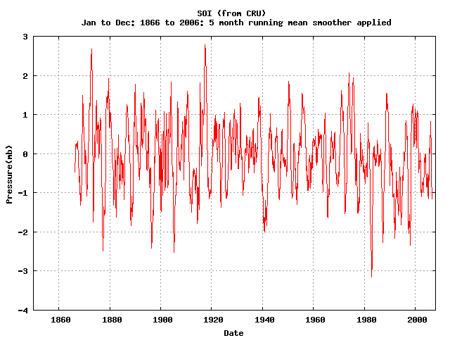
•  Time Series: SOI
  Choose in atlas:
  1. For variable: SOI
  2. For type: Plot
  3. 5 month running mean
  4. For variable: Anomaly
  5. For time: Jan 1920 to Dec 2000
•  Correlations: SOI
  Choose in page
  1. For variable: Tahiti SLP
  2. For variable: Darwin SLP
  3. For type: Correlation
  4. For time: Jan 1920 to Dec 2000
  Also try SOI and other locations in the tropics. Change the time range. Change the seasons by changing the months used. Do an annual average.
•  Map SLP anomalies Jan 1983
  Choose in atlas:
  1. For statistic: anomaly
  2. For variable: Sea Level Pressure
  3. For type: lat by lon
  4. For time: Jan 1983
  5. For options: color fill
  6. For latitude: 50N to 50S
  7. For Longitude: 20E to 340E
 
• Precipitation rates over India in July; long term mean.
  Choose in atlas:
  1. For statistic: longterm monthly mean
  2. For variable: precipitation rate
  3. For type:lat by lon
  4. For time: July
  5. For latitude: 0N to 40N
  6. For longitude: 45E and 100E
  7. For options: color fill and reverse color bar
 
• Precipitation rates over India in January; long term mean.
  Choose in atlas:
  1. For statistic: longterm monthly mean
  2. For variable: precipitation rate
  3. For type:lat by lon
  4. For time: July
  5. For latitude: 0N to 40N
  6. For longitude: 45E and 100E
  7. For options: color fill and reverse color bar
 
• Annual time series of precipitation rates over India. (not in talk but shows annual cycle very well).Choose:
  1. For statistic: longterm monthly mean
  2. For variable: precipitation rate
  3. For type:lat by time
  4. For time: Jan to Dec
  5. For latitude: 0N to 40N
  6. For longitude: 60E to 100E
  7. For options: color fill and reverse color bar

 

• Wind flow in June and January
  Choose:
  1. For statistic: long term monthly mean
  2. For variable: wind vectors
  3. For type: lat by lon
  4. For time:June (for second plot choose January)
  5. For level: 1000mb (near the surface)
  6. For latitude: 0N to 40N
  7. For longitude: 60E to 100E
  8. For plot options: solid fill
 
• Surface temperature over year over India
  1. For statistic: long term monthly mean
  2. For variable: air temperature
  3. For type: lat by time
  4. For time:Jan to Dec
  5. For latitude: 0N to 40N
  6. For longitude: 65E to 90E
  7. For plot options: solid fill , color reverse
 
• Surface temperature over year over India
  1. For statistic: long term monthly mean
  2. For variable: air temperature
  3. For type: lat by time
  4. For time:Jan to Dec
  5. For latitude: 0N to 40N
  6. For longitude: 65E to 90E
  7. For plot options: solid fill , color reverse
 
• Vertical motion over India (negative values are upward)
  1. For statistic: long term monthly mean
  2. For variable: air temperature
  3. For type: lat by level
  4. For time:June
  5. For latitude: 0N to 40N
  6. For longitude: 65E to 90E
  7. For plot options: solid fill , color reverse

El Nino examples

 
• SST plot
  1. For statistic: Longterm monthly mean
  2. For variable: Surface air temperature
  3. For type: lat by lon
  4. For time:Jan
  5. For latitude: 25S to 25N
  6. For longitude: 110E to 290E
  7. For plot options: solid fill
 
• SST anomaly plot 1982-83
  1. For statistic: Anomaly
  2. For variable: Surface air temperature
  3. For type: lat by lon
  4. For time: Dec 1982
  5. For latitude: 25S to 25N
  6. For longitude: 110E to 290E
  7. For plot options: solid fill
 
• local wind field plot
  1. For statistic: Long term monthly mean
  2. For variable: zonal wind
  3. For type: lat by lon
  4. For time: Dec to Feb
  5. For latitude: 25S to 25N
  6. For longitude: 110E to 290E
  7. For plot options: solid fill , color reverse
 
• local wind field anomaly plot
  1. For statistic: Anomaly
  2. For variable: zonal wind
  3. For type: lat by lon
  4. For time: Dec 1982 - Feb 1983
  5. For latitude: 25S to 25N
  6. For longitude: 110E to 290E
  7. For plot options: solid fill , color reverse
 
• Precipitation anomalies over globe
  1. For statistic: Long term monthly mean
  2. For variable: precipiation rate
  3. For type: lat by lon
  4. For time: Dec to Feb
  5. For latitude: 90S to 90N
  6. For longitude: 0E to 360E
  7. For plot options: solid fill , color reverse
 
• Precipitation over globe
  1. For statistic: Longterm mean
  2. For variable: precipiation rate
  3. For type: lat by lon
  4. For time: Dec 1982 to Fen 1983
  5. For latitude: 90S to 90N
  6. For longitude: 0E to 360E
  7. For plot options: solid fill , color reverse
 
• Precipitation anomalies over globe
  1. For statistic: Anomaly
  2. For variable: precipiation rate
  3. For type: lat by lon
  4. For time: Dec 1982 to Feb 1983
  5. For latitude: 90S to 90N
  6. For longitude: 0E to 360E
  7. For plot options: solid fill , color reverse

---