• Home
• Gridded Climate Data
• NARR
• Lambert Conformal Format

Lambert Conformal Format

In the netCDF file, the variables "lon" and "lat" contain those values for each of the coordinate pairs. Reading the data is simply a matter of reading the 349x277 array. Plotting may be harder as the grid is irregular. Below there are examples of how to plot the data in three commonly used packages. GrADS and NCL are free. You must buy a license for IDL.

and

GrADS

To plot in GrADS, you will need to interpolate. GrADS can interpolate data using a ddf like the one below. It is also possible to use GrADS to plot in the native grid directly. See the "Use PDEF For Displaying Pre-Projected Data With GrADS". You can also use a script from the GrADS standard library narropen.gs.

DSET ^air.197901.nc
DTYPE netcdf
TITLE NARR 4D field Lambert Conformal Conic projection
UNDEF -9999.0 missing_value
UNPACK scale_factor add_offset
PDEF 349 277 lcc 1 -145.5 1 1 50 50 -107 32463.41 32463.41
XDEF 205 linear 150 1
YDEF 85 linear 2 1
ZDEF 29 levels 1000, 975, 950, 925, 900, 875, 850, 825, 800, 775, 750, 725, 700,
 650, 600, 550, 500, 450, 400, 350, 300, 275, 250, 225, 200, 175, 150, 125, 100
tdef 1 linear 00z1jan2004 3hr
vars 3
air 29 t,z,y,x  air_temp
lat=>glat 0 y,x Latitude
lon=>glon 0 y,x Longitude
endvars

XDEF 615 linear 150 .333
YDEF 255 linear 2 .333

NCL

The NCAR command language NCL will plot the data. See particularly here to transform and here to see Lambert Conformal Conic described..

Sample Code:

Other examples may be found on this web page.

IDL

IDL will plot the data. Here is some skeleton-code that will help you set up your own code.

C set var to your variable, obtain scale and offset
C get time index for starting and stopping: itimestart, itimeend
C For 4-D variables (variables with levels) you will also need
C to get the netCDF variable level and you will need
C to have count and start be 4D with level being the 3rd array item.
*****************************************************************
nlons=349
nlats=277


vararray = fltarr(nlons,nlats)
vararryinin = intarr(nlons,nlats)
rlons  = fltarr(nlons,nlats)
rlats  = fltarr(nlons,nlats)

infile = 'yourfilename.nc'
nunit = ncdf_open(infile,/nowrite)
ivarid   = ncdf_varid(nunit,var)
ilatid   = ncdf_varid(nunit,'lat')
ilonid   = ncdf_varid(nunit,'lon')

NCDF_ATTGET,nunit,var,'add_offset',add_offset
NCDF_ATTGET,nunit,var,'scale_factor',xscale


for itime = itimestart,itimeend, 1 do begin
  offset   = [0,0,itime]
  count    = [nlons,nlats,1]

  ncdf_varget,nunit,ivarid,vararrayin,OFFSET=offset,$
    count = count
  vararray = vararray + (varscale*FLOAT(vararrayin) + varoffset)
endfor

ncdf_varget,nunit,ilatid,rlats,OFFSET=[0,0],$
  count = [nlons,nlats]
ncdf_varget,nunit,ilonid,rlons,OFFSET=[0,0],$
  count = [nlons,nlats]

ncdf_close, nunit

; ------------------------------------------------------------------
; plot the data
; ------------------------------------------------------------------

map_set,20.,60.,-95.,limit=[25,240,50,288],/advance,/conic,$
  title='yourtitle', /continents,/usa
contour,vararray,rlons,rlats,/cell_fill,/overplot,/noerase

Ferret

To plot in Ferret, use code similar to this. Note that the openDAP filename is used here.

yes? ! point to the OPeNDAP file name

yes? SET DATA "/cgi-bin/nph-nc/Datasets/NARR/monolevel/air.sfc.1979.nc"



yes? ! Draw the color plot using the curvilinear coordinates in the file

yes? SHADE/MODULO/HLIMITS=145:360/VLIMITS=0:90/LEVELS=50 air[L=1],lon,lat



yes? ! Run the land.jnl script included with Ferret to draw land outlines

yes? GO land.jnl 

MatLAB

In order to read NARR data into MATLAB we suggest that you use the mexnc and SNCTOOLS package at http://mexcdf.sourceforge.net/. Because the packed NARR data is roughly 500 MB per file, loading and unpacking the data can cause MATLAB to run out of memory. You can load only part of the file at a time by using:

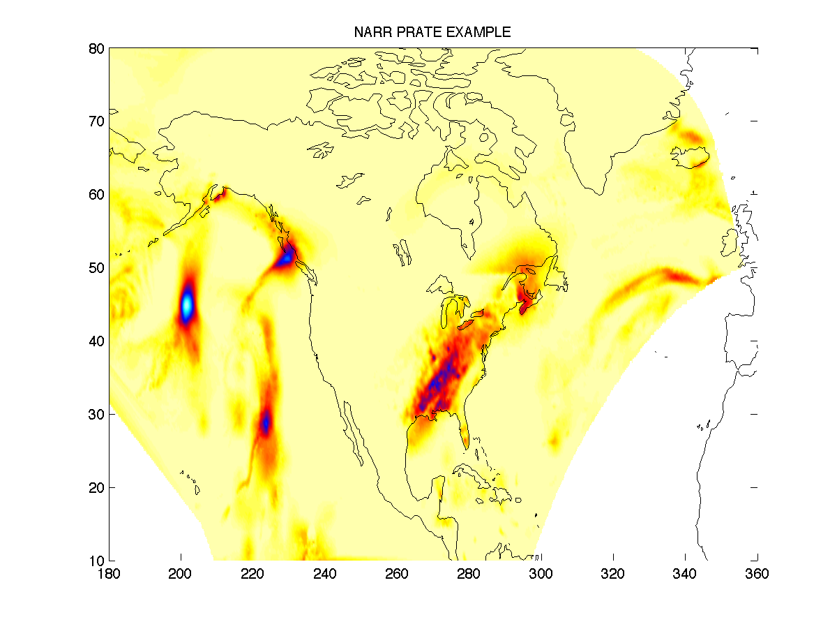
If the OpenDAP option is enabled for SNCTOOLS then a URL can be used in place of the filename. Alternatively, you can solve the memory problem by using NCO ( http://nco.sourceforge.net/ ) to extract a subset of the data before loading it into MATLAB. Here is a sample plot generated by interpolating the NARR data to a regular lat-lon grid:

p = nc_varget('prate.1979.nc','prate',[0 0 0],[10 -1 -1]);       %get all the gridpoints for the first ten timesteps in the file    pmean = double(squeeze(mean(p,1)));                              % Take the mean of these data over time    
nlat=nc_varget('/Datasets/NARR/monolevel/prate.1979.nc','lat');  % get the latitude and longitude coordinates
nlon=nc_varget('/Datasets/NARR/monolevel/prate.1979.nc','lon');   
nlon2 = nlon;nlon2(nlon<0) = nlon2(nlon<0)+360;                  % Make all longitudes have positive values   
x = 180:0.25:360;y=[10:0.25:80]';                                % Create a 1/4 degree lat-lon grid   
pint = griddata(double(nlon2),double(nlat),pmean,x,y,'linear');  % interpolate to this grid   
pcolor(x,y,pint);shading interp;colormap(1-jet.^2)               % make a pseudocolor plot    
load coast; 
hold on; 
plot(long+360,lat);
hold off                 % load MATLAB's coastal outlines and overlay the

If you have the mapping toolbox there is a much simpler and faster solution (sample output):

p = nc_varget('prate.1979.nc','prate',[0 0 0],[10 -1 -1])     
pmean = double(squeeze(mean(p,1)));    
nlat=nc_varget('/Datasets/NARR/monolevel/prate.1979.nc','lat');
nlon=nc_varget('/Datasets/NARR/monolevel/prate.1979.nc','lon');
axesm('eqdcylin','maplatlimit',[0 80],'maplonlimit',[150 0]);     % Create a cylindrical equidistant map   
pcolorm(nlat,nlon,pmean)                                          % pseudocolor plot "stretched" to the grid    
load coast
plotm(lat,long) 

Fortran/C