The fluxes in this graphic have a nominal spatial resolution of 1° longitude by 1° latitude, but with a strong influence of air-sea gas transfer velocity modeled at 3° x 2°. Optimization of air-sea flux in CarbonTracker is actually performed on the scale of 30 large regions representing areas of similar physical and biological processes (see thumbnail map on the left side of this page and ecoregion documentation). CarbonTracker estimates only the total weekly flux from each ocean region. The distribution of that total flux onto finer spatial and temporal scales such as those shown here depends on an underlying model of air-sea CO2 exchange. These finer scales are driven primarily by variability of sea-surface wind speed from the 3° x 2° atmospheric transport model. Fluxes on the ocean region scale, without this presumed finer-scale distribution, are shown in the figure at the bottom of this page. Ocean region uncertainties (Right). Uncertainty of the CarbonTracker estimate of air-sea exchange of CO2, averaged over the time period indicated. The quantity displayed is the one standard deviation uncertainty on estimated fluxes assuming Gaussian errors, in units of gC m-2 yr-1. Darker colors represent areas where the CarbonTracker flux estimate is less certain.
The uncertainties are originally available with weekly time resolution due to the inversion methodology. For monthly and annual averages, we show RMS averages from the weekly information. This scheme neglects temporal covariances. Uncertainties reported here are formal estimates from the inversion technique and do not include all sources of error. Flux uncertainties are among the most difficult quantities to compute, and care should be taken in their interpretation. Formal errors like these generally underestimate the true uncertainty, since they do not take into account all sources of error, like biases in simulated atmospheric transport.
The uncertainties in this graphic are uniformly distributed within each ecoregion (see thumbnail map on the left side of this page and ecoregion documentation). There is no assumed patterning of the uncertainty within ocean regions.
Note that fossil fuel emissions can occur over regions characterized as ocean. This is partly due to real emissions from international shipping, and partly due to emissions occurring in coastal land regions that are assigned to the ocean in our coarse 1x1 degree division scheme. The same is true for fossil fuel emissions over non-optimized regions such as ice, polar deserts, and inland seas.