|
Overview
Results
Resources
|
|
Documentation - CT2011_oi
|
|
|
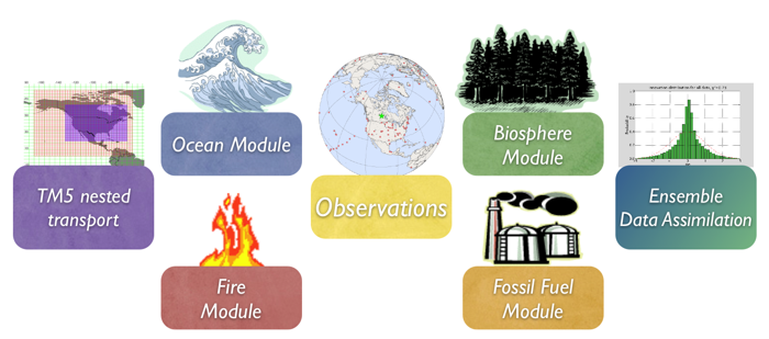
To learn more about a CarbonTracker component, click on one of the above images.
Or download the full PDF version for convenience.
|
|
1. Introduction
Data assimilation is the name of a process by which observations of
the 'state' of a system help to constrain the behavior of the system
in time. An example of one of the earliest applications of data
assimilation is the system in which the trajectory of a flying rocket
is constantly (and rapidly) adjusted based on information of its
current position, heading, speed, and other factors, to guide it to
its exact final destination. Another example of data assimilation is a
weather model that gets updated every few hours with measurements of
temperature and other variables, to improve the accuracy of its
forecast for the next day, and the next, and the next. Data
assimilation is usually a cyclical process, as estimates get refined
over time as more observations about the "truth" become
available. Mathematically, data assimilation can be done with any
number of techniques. For large systems, so-called variational and
ensemble techniques have gained most popularity. Because of the size
and complexity of the systems studied in most fields, data
assimilation projects inevitably include supercomputers that model the
known physics of a system. Success in guiding these models in time
often depends strongly on the number of observations available to
inform on the true system state.
In CarbonTracker, the model that describes the system contains
relatively simple descriptions of biospheric and oceanic CO2 exchange, as well as fossil fuel and fire
emissions. In time, we alter the behavior of this model by adjusting a
small set of parameters as described in the next section.
2. Detailed Description
The four surface flux modules drive instantaneous CO2 fluxes in CarbonTracker according to:
F(x, y, t) = λ • Fbio(x, y, t) + λ • Foce(x, y, t) + Fff(x, y, t) + Ffire(x, y, t)
Where λ represents a set of linear scaling factors applied to
the fluxes, to be estimated in the assimilation. These scaling factors
are the final product of our assimilation and together with the
modules determine the fluxes we present in CarbonTracker. Note that no
scaling factors are applied to the fossil fuel and fire modules.
2.1 Land-surface classification
The scaling factors λ are estimated for each week and assumed
constant over this period. Each scaling factor is associated with a
particular region of the global domain, and currently the geographical
distribution of the regions is fixed. The choice of regions is a
strong a-priori constraint on the resulting fluxes and should
be approached with care to avoid so-called "aggregation errors"
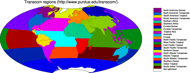
[Kaminski et al., 2001]. We chose an approach in which the ocean is divided
up into 30 large basins encompassing large-scale ocean circulation
features, as in the TransCom inversion study (e.g. Gurney et al.,
[2002]). The terrestrial biosphere is divided up according to
ecosystem type as well as geographical location. Thereto, each of the
11 TransCom land regions contains a maximum of 19 ecosystem types
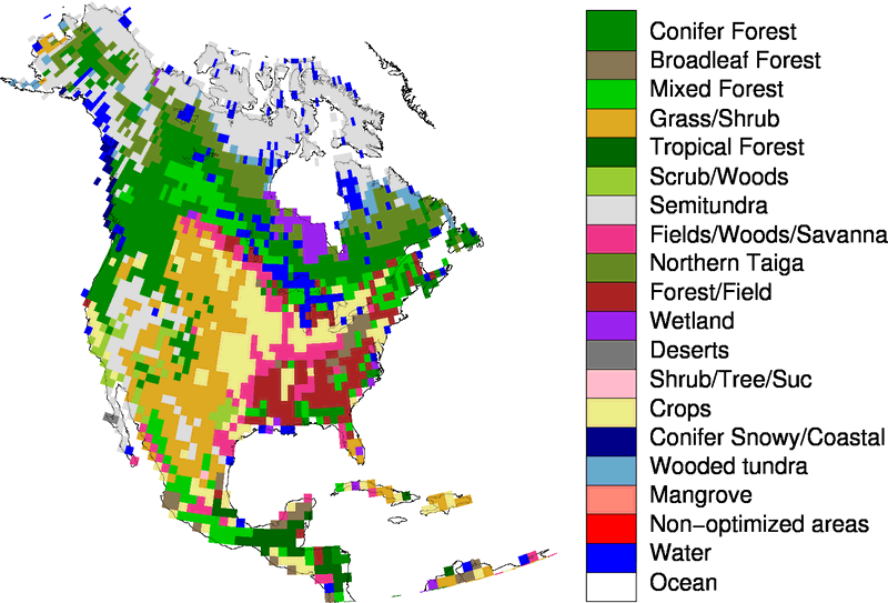
summarized in the table below. Figure 1 shows ecoregions for North
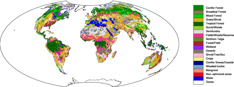
America (click here for global land
ecoregions). Note that there is currently no requirement for
ecoregions to be contiguous, and a single scaling factor can be
applied to the same vegetation type on both sides of a continent.
Further details on ecoregions can be found here.
|
|
Fig 1. CarbonTracker ecoregions in North America
|
Theoretically, this approach leads to a total number of 11*19+30=239
optimizable scaling factors λ each week, but the actual number
is 156 since not every ecosystem type is represented in each TransCom region, and because we
decided not to optimize parameters for ice-covered regions, inland
water bodies, and desert. The total flux coming out of these last
regions is negligibly small. It is important to note that even though
only one parameter is available to scale, for instance, the flux from
coniferous forests in Boreal North America, each 1° x 1° grid
box predominantly covered by coniferous forests will have a different
flux F(x,y,t) depending on local temperature, radiation, and CASA
modeled monthly mean flux.
Ecosystem types considered on 1° x 1° for the terrestrial flux
inversions is based on Olson, [1992]. Note that we have adjusted the
original 29 categories into only 19 regions. This was done mainly to
fill the unused categories 16,17, and 18, and to group the similar
(from our perspective) categories 23-26+29. The table below shows each
vegetation category considered. Percentages indicate the area
associated with each category for North America rounded to one
decimal.
Ecosystem Types
| category | Olson V 1.3a | Percentage area
|
|---|
| 1 | Conifer Forest | 19.0%
| | 2 | Broadleaf Forest | 1.3%
| | 3 | Mixed Forest | 7.5%
| | 4 | Grass/Shrub | 12.6%
| | 5 | Tropical Forest | 0.3%
| | 6 | Scrub/Woods | 2.1%
| | 7 | Semitundra | 19.4%
| | 8 | Fields/Woods/Savanna | 4.9%
| | 9 | Northern Taiga | 8.1%
| | 10 | Forest/Field | 6.3%
| | 11 | Wetland | 1.7%
| | 12 | Deserts | 0.1%
| | 13 | Shrub/Tree/Suc | 0.1%
| | 14 | Crops | 9.7%
| | 15 | Conifer Snowy/Coastal | 0.4%
| | 16 | Wooded tundra | 1.7%
| | 17 | Mangrove | 0.0%
| | 18 | Non-optimized areas (ice, polar desert, inland seas) | 0.0%
| | 19 | Water | 4.9%
|
Each 1° x 1° pixel of our domain was assigned one of the
categories above bases on the Olson category that was most prevalent
in the 0.5° x 0.5° underlying area.
2.2 Ensemble Size and Localization
The ensemble system used to solve for the scalar multiplication
factors is similar to that in Peters et al. [2005] and based on the
square root ensemble Kalman filter of Whitaker and Hamill, [2002]. We
have restricted the length of the smoother window to only five weeks
as we found the derived flux patterns within North America to be
robustly resolved well within that time. We caution the CarbonTracker
users that although the North American flux results were found to be
robust after five weeks, regions of the world with less dense
observational coverage (the tropics, Southern Hemisphere, and parts of
Asia) are likely to be poorly observable even after more than a month
of transport and therefore less robustly resolved. Although longer
assimilation windows, or long prior covariance length-scales, could
potentially help to constrain larger scale emission totals from such
areas, we focus our analysis here on a region more directly
constrained by real atmospheric observations.
Ensemble statistics are created from 150 ensemble members, each with
its own background CO2 concentration field to
represent the time history (and thus covariances) of the filter. To
dampen spurious noise due to the approximation of the covariance
matrix, we apply localization [Houtekamer and Mitchell, 1998] for
non-MBL sites only. This ensures that tall-tower observations within
North America do not inform on for instance tropical African fluxes,
unless a very robust signal is found. In contrast, MBL sites with a
known large footprint and strong capacity to see integrated flux
signals are not localized. Localization is based on the linear
correlation coefficient between the 150 parameter deviations and 150
observation deviations for each parameter. If the relationship
between a parameter deviation and its modeled observational impact is
statistically significant, then that relationship is used to modify
parameters. Otherwise, the relationship is assumed to be spurious
noise due to the numerical approximation of the covariance matrix by
the limited ensemble. We accept relationships that reach 95%
significance in a student's T-test with a two-tailed probability
distribution.
2.3 Dynamical Model
In CarbonTracker, the dynamical model is applied to the mean parameter
values λ as:
λ tb =
(λ t-2a + λ t-1
a + λ p ) ⁄ 3.0
Where "a" refers to analyzed quantities from previous steps, "b"
refers to the background values for the new step, and "p" refers to
real a-priori determined values that are fixed in time and
chosen as part of the inversion set-up. Physically, this model
describes that parameter values λ for a new time step are
chosen as a combination between optimized values from the two previous
time steps, and a fixed prior value. This operation is similar to the
simple persistence forecast used in Peters et al. [2005], but
represents a smoothing over three time steps thus dampening variations
in the forecast of λ b in time. The
inclusion of the prior term λ p acts
as a regularization [Baker et al., 2006] and ensures that the
parameters in our system will eventually revert back to predetermined
prior values when there is no information coming from the
observations. Note that our dynamical model equation does not include
an error term on the dynamical model, for the simple reason that we
don't know the error of this model. This is reflected in the treatment
of covariance, which is always set to a prior covariance structure and
not forecast with our dynamical model.
3 Covariance Structure
Prior values for λ p are all 1.0 to
yield fluxes that are unchanged from their values predicted in our
modules. The prior covariance structure Pp
describes the magnitude of the uncertainty on each parameter, plus
their correlation in space. The latter is applied such that
correlations between the same ecosystem types in
different TransCom regions
decrease exponentially with distance (L=2000km), and thus assumes a
coupling between the behavior of the same ecosystems in close
proximity to one another (such as coniferous forests in Boreal and
Temperate North America). Furthermore, all ecosystems within
tropical TransCom regions are
coupled decreasing exponentially with distance since we do not believe
the current observing network can constrain tropical fluxes on
sub-continental scales, and want to prevent spurious compensating
source/sink pairs ("dipoles") to occur in the tropics.
In our standard assimilation, the chosen standard deviation is 80% on
land parameters. All parameters have the same variance within the land
or ocean domain. Because the parameters multiply the net-flux though,
ecosystems with larger weekly mean net fluxes have a larger variance
in absolute flux magnitude.
3.1 Multiple prior models
In Bayesian estimation systems like CarbonTracker, there is a
potential for bias from a flux prior to propagate through the
inversion system to the final result. It is difficult to quantify
this effect, and as a result it is generally considered a precondition
that flux priors be unbiased. We cannot guarantee this for any of our
fluxes, be they the prior estimates for terrestrial or oceanic
exchange, or the presumed wildfire and fossil fuel emissions. In
order to explicitly quantify the impact of prior bias on our solution,
in CT2011 CT2011_oi we present the result of a multi-model prior suite of
inversions. We have used two terrestrial flux priors, two air-sea
exchange priors one air-sea exchange prior, and two estimates of imposed fossil fuel emissions in
a three-way factorial design experiment. This has resulted in eight four
individual inversions, each using a unique combination of priors and
conducted independently according to the methods described above. We
present as a final result the mean flux across this suite of
inversions and the atmospheric CO2
distribution resulting from applying these mean fluxes to our
atmospheric transport model. Each of the priors is described in
detail on its corresponding documentation page (fossil,
land,
ocean).
Notice: CT2011_oi does not use the
"climatological" ocean prior.
After we released CarbonTracker 2011, a significant bug was discovered
in our atmospheric transport model. We have corrected the bug and are
releasing revised results under the release name "CT2011_oi". One
consequence of this problem is that the four inversions using the
climatological ocean flux prior were faulty. They have been removed
from the inversion suite in CT2011_oi. Use of the original CT2011
results is strongly discouraged. Details can be
found at this link.
|
|
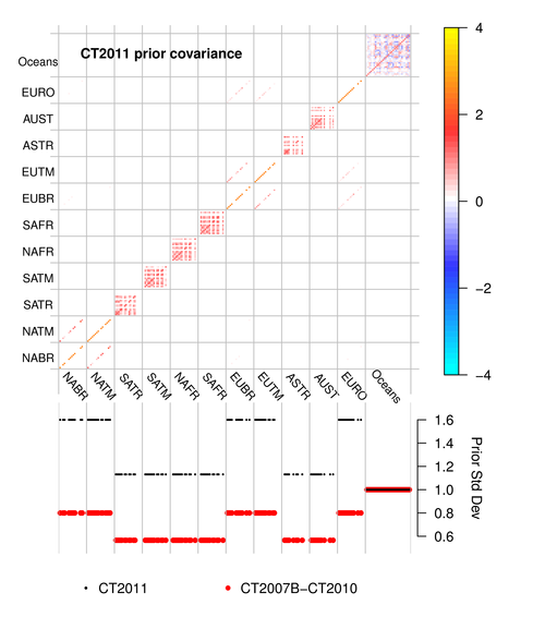
Fig 2. CT2011_oi prior covariance structure. The prior
covariance matrix (top panel) and the square root of diagonal members
of this matrix (bottom panel). Covariance matrix quantities are
dimensionless squared scaling factors, and the bottom panel is the
square root of this. TransCom land
regions form the first 11 large divisions on the axes here. As
described above, each of those regions contains 19 potential
ecosystems. Correlations between similar ecosystems in proximate
Transcom regions are visible in North America (e.g. NABR and NATM, the
boreal and temperate North American regions) and Eurasia. Within
tropical Transcom regions, however, differing ecosystems are assigned
a non-zero prior covariance, which is visible here as red block-like
structures on the diagonal within, for example, the South America
Tropical (SATR) Transcom region. Ocean regions have a more
complicated covariance structure that depends on which prior is used;
the structure shown here is that of
the ocean inversion flux
prior. The lower panel of this diagram compares the on-diagonal
elements of the prior covariance matrix by plotting their square
roots. The resulting standard deviations are directly comparable to
the percentages discussed in section 3 above; 0.8 is equivalent to
80%. The retuning of the covariance matrix for CT2011_oi's
multiple-prior simulation is made evident by also showing these values
from previous CarbonTracker releases in red.
|
3.2 Posterior Uncertainties in CarbonTracker
The formal "internal" error estimates produced by CarbonTracker are
unrealistically large. This is largely a result of the relatively
short assimilation window in CarbonTracker, along with a dynamical
model that introduces a fresh prior covariance matrix with every new
week entering the assimilation window. This five-week window
effectively inhibits the formation of anticorrelations ("dipoles") in
flux estimates, and does little to reduce the confidence interval on
prior fluxes.
The temporal truncation in CarbonTracker imposed by its five-week
assimilation window tends to yield regional flux estimates that are
largely uncorrelated with those from other regions. A consequence of
this feature is that uncertainties in CarbonTracker tend to increase
as larger regions are considered; regional errors mostly just add in
quadrature without any cancellation from dipole anticorrelation.
Whereas many inversions yield smaller errors as the spatial extent of
the region being considered increases, CarbonTracker acts in the
opposite fashion. This is perhaps most obvious in the estimate of
CarbonTracker's global
annual surface flux of carbon dioxide. While CT2011_oi estimates a
one-sigma error of more than 6 PgCyr-1 on its
global flux, this quantity is in actuality much more well-constrained.
This is evident from
CarbonTracker's excellent agreement
with observational estimates of atmospheric growth rate.
In CT2011_oi, error estimates are about a factor of two larger than in
previous releases, mainly due to the retuning of the land prior
covariance discussed above. However, uncertainties presented for
CT2011_oi take into account not only the "internal" flux uncertainty
generated by a single inversion, but also the across-model "external"
uncertainty representing the spread of the inversion models due to the
choice of prior flux.
4. Further Reading
|
|
