|
Information
Results
Get Involved
Resources
|
|
|
|
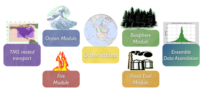
To learn more about a CarbonTracker component, click on one of the above images.
Or download the full PDF version for convenience.
|
|
1. Introduction
The biospheric component of the terrrestrial carbon cycle consists of all the
carbon stored in 'biomass' around us. This includes trees, shrubs,
grasses, carbon within soils, dead wood, and leaf litter. Such
reservoirs of carbon can exchange CO2 with
the atmosphere. Exchange starts when plants take up CO2 during their growing season through the process
called photosynthesis (uptake). Most of this carbon is released back
to the atmosphere throughout the year through a process called
respiration (release). This includes both the decay of dead wood and
litter and the metabolic respiration of living plants. Of course,
plants can also return carbon to the atmosphere when they burn, as
described our fire emissions
module documentation. Even though the yearly sum of uptake and
release of carbon amounts to a relatively small number (a few
petagrams (one Pg=1015 g)) of carbon per
year, the flow of carbon each way is as large as 120 PgC each
year. This is why the net result of these flows needs to be monitored
in a system such as ours. It is also the reason we need a good
physical description (model) of these flows of carbon. After all, from
the atmospheric measurements we can only see the small net sum of the
large two-way streams (gross fluxes). Information on what the
biospheric fluxes are doing in each season, and in every location on
Earth is derived from a specialized biosphere model, and fed into our
system as a first guess, to be refined by our assimilation procedure.
2. Detailed Description
The biosphere model currently used in CarbonTracker is the
Carnegie-Ames Stanford Approach (CASA) biogeochemical model. This
model calculates global carbon fluxes using input from weather models
to drive biophysical processes, as well as satellite observed
Normalized Difference Vegetation Index (NDVI) to track plant
phenology. The version of CASA model output used so far was driven by
year specific weather and satellite observations, and including the
effects of fires on photosynthesis and respiration (see van der Werf
et al., [2006] and Giglio et al., [2006]). This simulation gives
0.5° x 0.5° global fluxes on a monthly time resolution.
Net Ecosystem Exchange (NEE) is re-created from the monthly mean CASA
Net Primary Production (NPP) and ecosystem respiration (RE). Higher frequency variations (diurnal, synoptic)
are added to Gross Primary Production (GPP=2*NPP) and RE(=NEE-GPP) fluxes every 3 hours using a simple
temperature Q10 relationship assuming a
global Q10 value of 1.5 for respiration, and
a linear scaling of photosynthesis with solar radiation. The procedure
is very similar, but NOT identical to the procedure in Olsen
and Randerson [2004] and based on ECMWF analyzed meteorology. Note
that the introduction of 3-hourly variability conserves the monthly
mean NEE from the CASA model. Instantaneous NEE for each 3-hour
interval is thus created as:
NEE(t) = GPP(I, t) + RE(T, t)
GPP(t) = I(t) * (∑(GPP) / ∑(I))
RE(t) = Q10(t) * (∑(RE) / ∑(Q10))
Q10(t) = 1.5((T2m-T0) / 10.0)
where T=2 meter temperature, I=incoming solar radiation, t=time, and
summations are done over one month in time, per gridbox. The
instantaneous fluxes yielded realistic diurnal cycles when used in the
TransCom Continuous experiment.
|
|
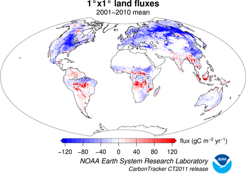
Fig 1. Map of optimized global biosphere fluxes. The pattern of net ecosystem exchange (NEE)
of CO2 of the land biosphere averaged over
the time period indicated, as estimated by CarbonTracker. This NEE
represents land-to-atmosphere carbon exchange from photosynthesis and
respiration in terrestrial ecosystems, and a contribution from
fires. It does not include fossil fuel emissions. Negative fluxes
(blue colors) represent CO2 uptake by the
land biosphere, whereas positive fluxes (red colors) indicate regions
in which the land biosphere is a net source of CO2 to the atmosphere. Units are gC m-2 yr-1.
|
CarbonTracker uses fluxes from CASA runs for the GFED project as its
first guess for terrestrial biosphere fluxes. We have found a
significantly better match to observations when using this output
compared to the fluxes from a neutral biosphere simulation. Prior to
CT2010, we used version 2 of the CASA-GFED model, which is driven by
AVHRR NDVI,
scaled to represent MODIS fPAR. Recently the GFED team has
transitioned to version 3.1 of their model, driven directly by MODIS
fPAR. We have found that the newer CASA-GFEDv3 product has a
smaller seasonal cycle than the older CASA-GFEDv2.
The record of atmospheric CO2 calls for a
deeper terrestrial biosphere sink than that generally simulated by
forward models like CASA-GFED. This is manifested by a larger annual
cycle of terrestrial biosphere fluxes, and in particular a deeper
boreal summer uptake of carbon dioxide, in the posterior optimized
fluxes compared to the prior models (See Box 1). We call upon the atmospheric
CO2 observations to make this change, and in
order to handle these prior model differences the ensemble Kalman
filter's prior covariance model has been re-tuned. In
short, this prior uncertainty needs to comfortably span differences
among the terrestrial biosphere priors, the fossil fuel emissions
priors, and adjustments to fluxes required to bring model predictions
into agreement with observations. As a result, the land biosphere
prior uncertainty has been doubled in CT2011 in comparison to previous
releases. Details can be found on the assimilation scheme
documentation page.
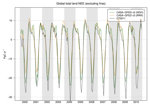
Box 1. Comparison of terrestrial biosphere flux priors
|
|
Time series of global-total terrestrial biosphere flux
between the two priors and the CT2011 posterior. Global
CO2 uptake by the land biosphere,
expressed in PgC yr-1, excluding
emissions by wildfire. Positive flux represents emission of
CO2 to the atmosphere, and the negative
fluxes indicate times when the land biosphere is a sink of
CO2. While both priors manifest
similar annual cycles of uptake in boreal summer balanced by
emission in boreal winter, the GFED3 prior (tan) has an annual
cycle that is about 10% smaller than that of GFED2 (green).
Optimization against atmospheric CO2
data requires a larger land sink than in either prior, which
effectively requires a deeper annual cycle. This is shown by
the CT2011 posterior (black).
|
|
|
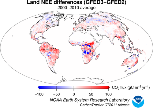
Differences in long-term mean terrestrial biosphere fluxes
between the two priors. Red indicates areas where the GFED3
prior has less terrestrial uptake (or more outgassing to the
atmosphere) than the GFED2 prior, and blue represents the
opposite. Units are gC m-2
yr-1.
|
Unlike CT2010, CarbonTracker 2011 is a full reanalysis of the
2000-2010 period using new fossil fuel emissions, CASA-GFEDv3 fire
emissions, and first-guess biosphere model fluxes derived from
CASA-GFEDv2 for 4 of our inversions, and from CASA-GFEDv3 for the
remaining 4 inversions.
Due to the inclusion of fires, inter-annual variability in weather and
NDVI (or fPAR), the fluxes for North America start with a small net
flux even when no assimilation is done. This flux ranges from
0.05 PgC yr-1 of release, to
0.15 PgC yr-1 of uptake.
3. Further Reading
|
|
